Experiments and data
Posted on 2019 / 12 / 09 in ChSU
Greetings to everyone who interested in this topic!
This section is dedicated to the basics of experiment planning and analysis of the acquired data. This is the core of any scientific and analytical work. However, I do not see much difference in what kind of science or discipline it will be. In fact, we conduct experiments and process data all the time. So, I will try to make this course as useful and meaningful as possible, regardless of the field of application. After all, we are all scientists and engineers in ordinary life (the question is: good or bad?). We solve various optimization tasks (e.g. how to get a higher salary), accumulate data through observations and draw conclusions from our own experience.
The goal of the course is to develop a general theoretical and practical vision of science, data and experiment.
Main objectives are:
- Show the terminology and logic of experiments in science.
- Describe the features of the experiment in terms of the investigated factors.
- Define effective ways of carrying out the experiment and obtaining information in order to optimize the system response.
- Provide an introduction to statistics and processing of the results.
- Introduce the building of linear regression models.
- Consider and solve some problems and examples, which are related to the course topic.
Many tasks and definitions in this module are taken from excellent courses from [coursera.org] (https://www.coursera.org/) and [stepic.org] (https://stepik.org/) (more in the reference list), as well as from various analytical chemistry's textbooks and manuals. All presented material has been studied, structured and redesigned based on my own experience and reflects my subjective point of view.
1. Introduction. Science and scientific approach
Well, science and scientific approach, what is this?
Science - systematic representation about structure and organization of all "knowledge" (information) about our life and Universe with the possibility of verification and prediction.
As we know from ancient Greek's philosophy, we have only two option to study our environment: the observation and the experiment (I really can't see any controversies about this assumption in nowadays).
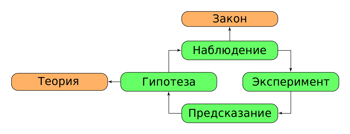
The scientific activity can be described as "data collection through observations and experiments". Besides, they are constantly updated, systematized and analysed. The consequence is the acquisition (synthesis) of new knowledge and laws of our World. In other words, on the basis of data, we create theories and hypotheses that are confirmed/confronted by observations or experiments. Thus, we can assume the following cycle of scientific cognition (Fig. 1, Table 1).
|
Fig. 1. Relations in "science cycle". |
Table 1. The terms of scientific study
| apply to unit or small amount | apply to all cases | |
|---|---|---|
| describe what is happening | observation | law |
| describe why it is happening | hypothesis | theory |
As a general rule, in any science we will work on hypotheses and theories, operating with laws and observations (data).
At the same time, we should not forget that the basic tool of description and classification of any phenomenon is mathematics. To work effectively in the modern world, we need one more tool - programming. I advise you not to forget about it and then your competence will be high.
The experiment itself is an essential part of science and our lives. It is the planned observation (made for a purpose). We all conduct experiments in our daily lives. As one teacher said, if you stop experimenting, you are disappointed in life. And that means it's time to start any movement and experiment again.
The challenge. Think about it, have you experimented recently? What does an experiment mean to you?
Here's a good example of an experiment. Let us grow the plant in front of our monitor and set the goal to optimize its growth. First of all, we should analyze how the growth is expressed: length, number of leaves, weight, etc.. Then, you need to determine factors (or features) that can affect the length of the plant: water amount for irrigation, irrigation frequency, soil type, plant pot type, fertilizer type, fertilizer amount, light, temperature, etc...
Thus, we have obtained quite a few factors, which can affect to our system. We need to understand which factors (or its combination) will allow us to achieve the goal.
From this example, we can see what we will face next. We will have to plan and describe our experiments, as well as process the data and demonstrate whether it is statistically correct (representative).
To successfully plan an experiment we need to understand the theory of examined field of knowledge as well as its terminology (in order to set goals and define factors correctly). In addition, it is important to use the scientific cycle, which is described earlier. Shall we begin?
2. Experiments, systems and factors
2.1 Introduction and terminology
During the experiment, our goal is outcome(s), what we want to know/optimize/represent in numeric form (i.e. measured). Synonym of the outcome is response of the system.
Factors (features, variables) -variable properties, which are supposed to determine the result of the experiment.
All experiments should have at least 1 changeable (and measurable) factor. And the more number of factors we take into account, the better (in the general case).
The factors themselves are divided into:
- quantitative (numeric) - can be measured and compared (e.g. ordered by increasing/decreasing);
- qualitative (categorical, nominal) - are determine the type of objects, but cannot be numeric compare.
Sometimes there are also the rank factors, which determine the type as qualitative variables, but they can be compared to each other (for example, the place in the competition). However, only quantitative or qualitative values are used to analyze results in major cases. Rank values are used to calculate various statistical criteria.
Example. Let's consider a classical example of building an experiment and processing its results. We want to increase the profit of the store (\(= \text{revenue} - \text{expenses}\)) and we think that it will be influenced by 2 factors: the illumination of the room (we can set the dimmer at 50 \% and 75 \%) and the price of goods (let's say 7.79 \\( or 8.49 \\)). So we are faced with a two-factor experiment.
Note that such experiment should be carried out 4 times (for example, every Monday). It's not enough just to change one feature one time (3 experiments), you need to add one more - when both features change at once. It will 2 times increase quantity of the received information and allow to compare influence of both features on experiment result. Further we will see the reason why.
While planning the experiment, we should use a special table (Table 2). The sequence of data in the table are called the standard test sequence.
Table 2. Example of the experiment data
| No | real No | Dimmer, % | Price | Profit, $ |
|---|---|---|---|---|
| 1 | 3 | 50 | Low | 490 |
| 2 | 1 | 75 | Low | 570 |
| 3 | 4 | 50 | High | 370 |
| 4 | 2 | 75 | High | 450 |
Once we've recorded the results, we can start analyzing them. For example, the effect of light brightness at low price is 80 \\( (difference between dim and bright light). The same effect at a high price is 80 \\). So, we observe the increase of profit by 80 \$ from the illumination effect. You can see that the effect is the same at different price levels.
Same for the price effect: in dim light it goes to 120 \\(, in bright light it goes to 120 \\). Thus, when the price of the goods increases, the profit falls (in our case only).
The challenge. What do you think might go wrong? What factors we didn't take into consideration and what else might affect profit? Is our experiment reproducible (will we get the same results just repeating our experiment)?
It is interesting that for the above example, many people would not do 4 experiments, but 3. As the first experiment, they would choose low light and low price. Further, they would carry out the second experiment (increase the brightness of light at a constant price). Then, they would return to an initial point and would carry out the third experiment (increase only the price).
A lot of people will think that's the way to do experiments. Because you only change one factor per time. You were trained to do that at school and university. You can only change one parameter at a time. But in general, you don't have to do that!
If you limit yourself to these three experiments, you will get only one evaluation of the effect of light and only one evaluation of the effect of price. However, by carry out one more experiment we will be able to evaluate both effects twice (when both factors are increased). In total, we will get two estimates of illumination effect and two estimates of price effect on profit. Therefore, by adding just one additional experiment, we will actually double the received information.
Note. We have described a so-called "full factor experiment". However, the example of a "fixed" experiment approach (when we change only one factor with fixed other factors) is very common in analytical chemistry. In case of calibration line, we change only one variable (analytical signal) under fixed conditions and calculate only one response (concentration). Why we can do this? What additional experimental work needs to be done before it is possible to fix other factors?
For further study we will need a number of terms and the concept of measurement error.
The generation of the set of our object observations is measurement process. The recording of observation in certain unit is quantitative analysis/the measurement (it is comparison with the established standard, e.g. when we measure something with a ruler). Thus, a quantitative measurement is a recorded result of a comparison in a certain units. Qualitative analysis is simply a relative result of comparison without units (more or less, there is an object or not). Sometimes you can read about semi-quantitative analysis, which is not very precise quantitative analysis (but better than nothing).
2.1.1 Accuracy and precision (repeatability)
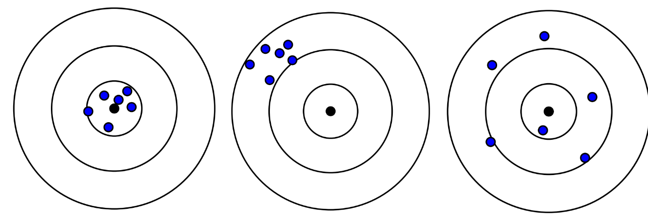
We have arrived at the basic concepts of experimental data processing: accuracy and precision. These terms can be better explained by the analogy with targets for shooting (Fig. 2).
|
Fig. 2. Examples of accurate and precise shooting. From left to right: accurate and precise, not accurate but "precise", and not precise but accurate in average. |
Accuracy indicates the closeness of the obtained result to the absolute value, and precise indicates closeness to the previous obtained result. Precise and accuracy are evaluated using a very important and useful tool - statistics (field of mathematics).
To estimate the accuracy of the obtained result, we can use the concept of absolute and relative error.
Absolute error can be measured as \(a = x_{true} − x_{our}\), where \(x_{true}\) - the true value (usually we didn't know it and use referent or average values), \(x_{our}\) - measured value. As you can see, the absolute error measured in the same unit as x.
Relative error can be measured as \(\Delta = \frac{x_{true} - x_{our}}{x_{true}}\) and use relative unit or percent (if we multiply it with 100 \%).
Precision is defined a bit more complex and we will return to it in part 3 of this course.
It is worth saying that there are only 2 nature of error: random (due to the statistical nature of measurements, which is always present in our imperfect world) and systematic (due to the action of some constant disturbance force, which can be corrected).
Note. The prevalence of a "fixed" approach in analytical chemistry is caused by the fact that it provides greater accuracy and precision of the obtained results. However, before selecting the most significant factor and fixing all the others, it is necessary to carefully examine the system. This is what factor experiments are used for. In addition, factor experiment dominates in other fields of knowledge, including chemical technology.
2.1.2 Some words about the rules for result presentation
The significant digits and round rules are important concept of any nature sciences. In other words, it is necessary to show how many digits in the result have real physical justification. Other digits should be dropped (we will not lose the accuracy).
The number of significant digits determines the error of the experiment (and vice versa, the measurement result is rounded to the same digit as the absolute error with one significant digit).
Example. If, due to the experiment we get 100.1, 99.8 and 100.2 M of concentration for standard sample with justified concentration of 100.0 M, then average absolute error is: \(\frac{\sum |x_i - 100|}{3} = \frac{0.1 + 0.2 + 0.2}{3} = 0.16666.. \approx 0.2\). Thus, our average experimental value is: \(\frac{100.1 + 99.8 + 100.2}{3} = 100.0333... = 100.0\).
Such result is usually wrote as \(100.0 \pm 0.2\). Last digit is not precisely define and can take any value within the limits of the experimental error \(x \in [99.8; 100.2]\).
The significant numbers are very useful for the natural sciences. They allow us to simplify some stages of the experiment and make it more reproducible. They also can show our colleagues the accuracy of our research. For example, if we know the accuracy for our experiment (e.g. 4 significant numbers for 10.00 M), then we can weight our reagent with that accuracy (4 significant numbers also, like 10.50 g, without 4 digits after dot).
We show you below some rules for significant digits. If you want to understand and remember it, you have to think about error concepts. The last significant digit contains the absolute error of experiment.
- Each digit other than 0 is significant (for example, 237 - 3 significant digits, 129.7 - 4 significant digits).
- 0 before not 0 digits - not significant (0.0165 - 3 significant digits). In this case it is better to apply "scientific" or exponential number record: \(1.65 \cdot 10^{-1}\).
- 0 to decimal point - you can't say for sure, that's not how a scientist should write (you shouldn't write 10, you should write it as \(1.0 \cdot 10\)). Unfortunately, I meet such a record very often in my practice. If you found such record too (e.g. 3700 units), then a person, who made it is not familiar with the practice of significant digits and just rounded experimental result up to the integer. You can only drop this number or analyze the experiment and set the number of significant digits by yourself (use the weighting accuracy or absolute error).
- In other cases 0 is significant (85,950 - 5 significant digits, 12.06 - 4 significant digits).
Note. The scientific (exponential) record of a number always involves a single digit to the decimal point and the exact indication of significant digits after it (e.g. \(1.650 \cdot 10^{-10}\) or \(2.740 \cdot 10^{5}\)). I strongly recommend you always using it in experimental practice.
Example. Mass of sample is 0.1 g. If you had weighted it with analytical scale with \(\pm 0.0001\) g error, then you has to write your result as \(0.1000 = 1.000 \cdot 10^{-1}\) g.
Moreover, there are some arithmetic rules for significant digits. They allows us to preserve physical sens in calculation and in finished result.
- Add/subtract - use absolute categories (number size is important). Leave as many digits after the decimal point as there are in the summand with the smallest number of decimal digits (i.e. accuracy is limited by the number, which have the bigger absolute uncertainty). Remember, the last significant digit carries an uncertainty, which limits everything else and when we add/subtract numbers such effect will be proportional to the size of number.
- Multiplication/division - use relative categories (at multiplication or division the uncertainty of the limiting number is proportionally transferred to the result). The number of significant digits of the result will be equal to the minimum number of significant digits of the participants (i.e. the accuracy is limited by the number, which have the bigger relative uncertainty). If the number of significant digits of participants are the same, the accuracy is limited by the number, which have the smallest mantissa (the absolute value, which is equal to all ordered digits of number).
Example. For \(0.0304 \times 5.43\) mantissa of 1st number is 304, and mantissa of second number is 543. So, the 0.0304 is number, which limit accuracy (it's relative error is bigger, then relative error of 5.43).
- Logarithmization - logarithmic number and mantissa (in case of logarithmization it is the result of logarithm) contain the same number of significant digits.
Example. Let's calculate the pH value of \(2.0 \cdot 10^{-3}\) M of HCl solution. The base of logarithm and 10's degree are the exact values. Then the result is:
Note, that due to the addition of an absolutely accurate value of 3, the final result have 3 significant digit - more, than the initial value (the absolute measurement error remained the same, but the relative error decreased).
- Exponentiation - multiplication of numbers with the same number of significant digits. The number of significant digits in the result will be the same as in initial value.
- Root of number - can be represented as a result in absolute degree, i.e. multiple multiplication of the result. The number of significant digits will thus remain the same as in the initial value.
- We follow the arithmetic order as in mathematics.
- To avoid accumulation of an error, the result is rounded only at the end of the whole calculation. In intermediate calculations we leave the number of significant digits + 1. In the final result, this additional digit is rounded up.
Note. The above calculation rules with significant digits are nothing but an approximation for the error of the result. For this reason, it is extremely unwise to perform many calculations for values with errors (especially exponentiation, taking the root and logarithms) - the more such operations, the more uncertain our final result is in reality. The arithmetical rules for significant digits can be strictly justified on the basis of the law of error propagation (but we will certainly not do it).
Note. The results of gravimetric and titrimetric determinations are in most cases recorded as numbers with 4 or 2 significant digits, which is related to the error of measurement of the mass of substances (e.g. \(\pm 0.0001\) g) and volumes of solutions (e.g. \(\pm 0.03\) ml). However, the number of significant digits strongly depends on the initial weight of the analyzing sample.
Note. Experimental result and its error should have the same digits after decimal dot (e.g. \(10.1 \pm 0.1\)).
Rules of rounding: * we round up to the number of significant digits (the last digit has an uncertainty); * if the rounded digit is more than five or less, round it up to the appropriate side; * if the rounded digit is 5, we round it up to the nearest even digit (if we need to round up only one digit 5: \(10.5 \approx 10\), but this is not the case if we round up 2 digits \(10.51 \approx 11\)); * do not round up intermediate calculations, leave the required number of significant digits + 1. * always remember that significant digits is an absolute measurement error of the value and you should work with them accordingly to described rules.
Example. Calculate the result:
2.2 Analysis of two-factor experiment
I hope, that I was able to show you how to record the results of experiments and convinced you about the importance of factor experiments in our lives. It's time to move on to studying and analyzing them.
Let's take the popcorn as an example. We will try to optimize the number of popped kernels. The good thing about this experiment is that you can repeat it at home. If you don't understand something, you can feel free to write to me or watch [the course] (https://www.coursera.org/learn/experimentation) where this experiment is analyzed in more detail.
Well, we have 2 investigated factors in such experiment. This factors can take 2 values each: A - heating time (160 and 200 s) and B - type of kernels (yellow and white). We can easily calculate that the number of experiments will be 4.
Note. In general, you can use the following formula: \(f^v = 2^2 = 4\), where \(f\) is the number of factors and \(v\) is the number of values, which each factor can have (according to another area of mathematics, combinatorics). In our case, we will always use the same number of levels for factors, consider it a kind of requirement for such plans of experiments.
Let us make a table of the experiment (Table 3) and denote - and + (low and high) level of factors (for the categorical factor order does not matter, we can choose any). Then for A: -: 160, +: 200, for B: -: White, +: Yellow.
Note. For informative results, it is important to:
- ** do not use extremes** for factors (otherwise they will be affected by many influences and will differ too much from each other, which will increase errors);
- ** always carry out experiments in random order!** This is the only way to get rid of the systematic error and the additional connections between the values.
Table 3. The results of a two-factor popcorn experiment.
| Standard order | Random order (real) | A - time \* | B - corn | Results |
|---|---|---|---|---|
| 1 2 3 4 |
3 1 4 2 |
- + - + |
- - + + |
52 74 62 80 |
* you should use the standard order for changing the level of factors. First, we change the 1st factor all the time, then we change the 2nd factor in matching order.
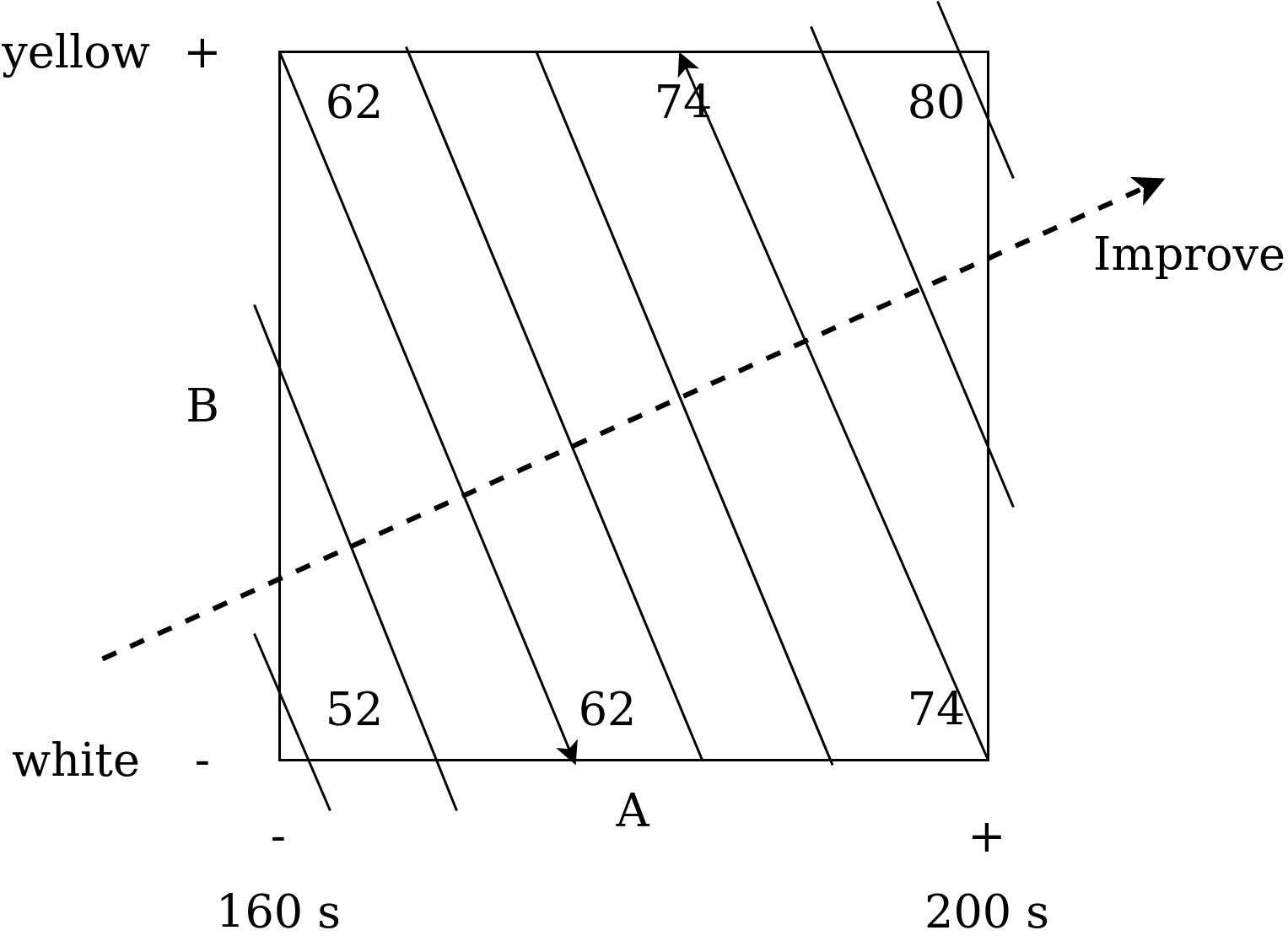
So, we have results, and now is good time for analysis. It's always a good idea to start with visualization (this is how we think). The visualization of factor experiment is called cube plot (graph, chart). It is shown in Fig. 3.
|
Fig. 3. Cube plot of 2 factor popcorn-experiment with isolines (contour lines). |
This plot shows the effect of each factors in corresponding square or cube corner (2 or 3 factor experiment respectively).
Let's start with heating time effect. When you increase the cooking time for yellow popcorn, the result increases from 62 to 80 popped kernels (PK). Therefore, we see an increase by 18 units. For white popcorn we see a rise from 52 to 74 PK, which is an increase by 22 units. So, on average, we see an increase by 20 units when the heating time increases from 160 to 200 seconds.
Then let's estimate the difference between the two types of popcorn. We fix heating time and look at the effect of switching from white to yellow popcorn: from 74 to 80 for 200 sec. and from 52 to 62 for 160 sec. On the average we see increase by 8 units during change from white to yellow popcorn. Make sure that your interpretation matches the cube chart. This visualization is very important for self-testing.
But besides the output, the cube plot also shows contour lines (contour plot or insolines). They indicate the area, which contain constant value of output (on 1 line the number of PK remain the same). They are drawn starting from any corner of the cubic diagram, which don't have maximum or minimum value. Then, equal value is searched on the opposite side of the square and line is draw. To check the curvature of the line, we need to calculate our fixed value for the middle of the scale (we see it later in this course).
Then we draw the second line in the same way for the value of 74. The others lines are drawn parallel to the obtained ones.
Thanks to the isolines, we can quickly understand where to start moving to optimize the result, i.e. towards to our goal. For example, if the goal is to maximize the number of popped kernels, then we need to move perpendicular to the isolines in the upper right corner. It means, that we should take yellow popcorn and increase the cooking time (which is quite intuitive from the cube plot).
Such an approach to optimization (using the isolines) helps us to define the way of carrying out the next experiment. The contour diagram is our gradient (path to maximize or minimize the output).
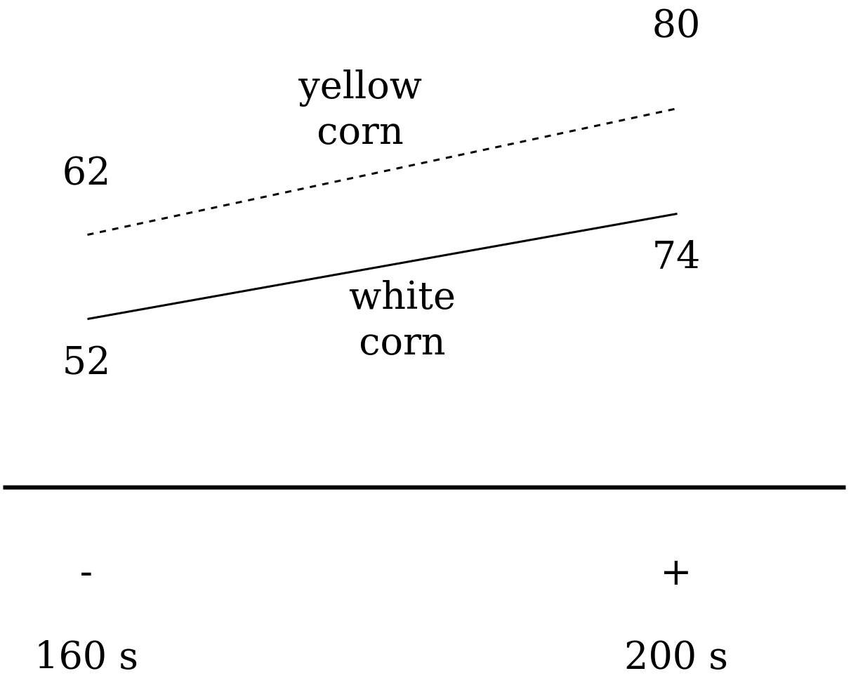
Moreover, we have another type of visualization, it is the diagram of interaction (Fig. 4).
|
Fig. 4. diagram of interaction for 2 factor popcorn experiment. |
Pay attention that these two lines are practically parallel, which means that there is practically no interaction in the examined system. The choice of a variable for the interaction diagram does not play a big role and we could choose another variable to be marked on the horizontal axis.
All the described methods of visualization do not require any software. You can use these visualization methods for both numerical and categorical factors. This shows the obvious advantage of such an approach to the experiment (we can quickly interpret the results using simple graphical tools, elementary mathematics and a sheet of paper).
Being that simple means, that the results can be easily shared with managers or colleagues at work.
2.3 Make a prediction
We discussed the example of planning, conducting and analyzing an experiment. But what does it give us? How can we present and use the obtained data? The answer is to build a prediction (model, regression equation). In our course, we will only consider linear models (with a few exceptions). Such models are the most universal (any smooth and monotonic function can be represented as a set of linear segments).
We discussed the example of planning, conducting and analyzing an experiment. But what does it give us? How can we present and use the obtained data? The answer is to build a prediction (model, regression equation). In our course, we will only consider linear models (with a few exceptions). Such models are the most universal (any smooth and monotonic function can be represented as a set of linear segments).
In case of our "popcorn experiment" (2-factor experiment), the obtained model consists of 3 parts:
where,
- \(a_0\) is the intercept that we expect to see when there is no effect (when the encoded factor values = 0). This coefficient is calculated as an average of 4 values in a cubic diagram (i.e. its center).
- \(a_1\) - coefficient of influence of factor A (its coded value), which depends on preparation time. It is calculated as the average normalized difference between the high and low values of the factor: \(a_1 = \frac{\frac{(80-62) + (74-52)}{2}}{2}\). Note that normalization involves the calculation of the coefficient for a unit change in the factor (i.e. from -1 to 0 or from 0 to +1), so we should divide the average by 2.
- \(a_2\) - Factor B coefficient, which depends on the type of grains. It is calculated similarly to point 2.
Considering the above description, our model will be:
The challenge. Check this model for different coded value of each factors.
2.4 Factors interaction
So far we have considered very ideal cases where factors have no interaction between each other and the target variable. However, this is frequently wrong.
Example. We try to wash our hands and conduct a 2-factor experiment: there is/no soap and warm/cold water. You may notice that the effect of warm water will increase when you use soap. And vice versa, the soap effect will be enhanced by using warm water. In other words, "interaction" indicates that the effect of one factor depends on the level of another factor.
Besides, these interactions are usually symmetrical. That means it makes no difference whether we wash our hands in warm water with soap or with soap in warm water, the result is the same.
The first indicator of the presence of interaction between factors is the asymmetry of lines in the interaction diagram or the curve form of isolines in the cubic diagram. If you observe such effects, it is double factors interaction (when the behavior of one variable is very depends on the level of the other one).
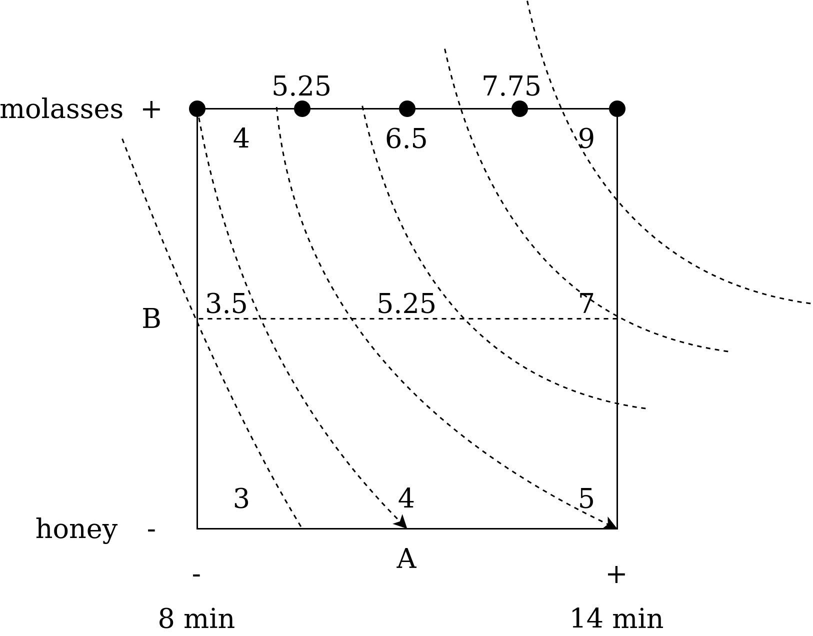
Let's consider the experiment in the figure 5 and calculate all the coefficients. The experiment involved analysis of the effect of baking time (factor A) and sugar type (factor B) on cookie taste (on a scale from 1 to 10).
|
Fig. 5. Cube plot for experiment with factors interaction. |
Note that the isolines are no longer parallel and should be presented in a curved form (once again, the result must be the same on the line). For this purpose I recommend you drawing an additional line in the center of the cube plot.
The expressed non-parallelism of lines indicates the presence of mutual influence of factors. Strictly speaking, when analyzing the experiment, it is always necessary to construct the model taking into account the mutual influence and exclude it only if the coefficient before this interaction is very small. Let us calculate the resulting model.
To build a model, the influence of each factor is calculated separately and in the same way as mention above. In case of interaction it is necessary to calculate changes at one fixed factor (sugar type) as an normalized averaged difference at high and low values of the feature: \(interaction = \frac{(9-4) - (5-3)}{2} = $1.5\). Let us check the symmetry of the influence by fixing another factor: \(interaction = \frac{(9-5)(4-3)}{2} = 1.5\). Thus, the influence is really symmetrical and equal (if not - take average value). Finally, our model is:
The challenge. Build interaction diagram and verify that there is an interaction. Check the accuracy of models prediction with and without interaction.
2.5 Three-factor experiment
Once we have mastered the basics of analyzing the results of the experiment, we can make the initial conditions more complicated. A new example is taken from textbook, which is called "Statistics for Experimenters: Design, Innovation, and Discovery". In the new experiment, an optimal combination of parameters is searched to reduce the pollutant in the waste water.
Once we have mastered the basics of analyzing the results of the experiment, we can make the initial conditions more complicated. A new example is taken from textbook, which is called ["Statistics for Experimentalists"] (https://www.amazon.com/Statistics-Experimenters-Design-Innovation-Discovery/dp/0471718130). In the new experiment, an optimal combination of parameters is searched to reduce the pollutant in the waste water of a wastewater treatment plant.
Three factors with 2 levels are considered. The first factor is C, which is a chemical compound (P and Q). The next factor is T (temperature), which is the water treatment temperature (\(72^o F, $100^o F\)). The last factor is S (stirring speed), which is mixing speed (200 or 400 rpm). Then the number of necessary experiments are:
where \(f\) is the number of factors and \(v\) is the number of values of each factor.
The result of the experiment is the number of pollutants measured in pounds.
Using the standard procedure of the experiment, we will make a table 4.
Table 4: Results of a three-factor experiment.
| Standard order | Random order (real) | C - chemical | T - time | S - stirring speed | Outcome |
|---|---|---|---|---|---|
| 1 2 3 4 5 6 7 8 |
6 2 5 3 7 1 8 4 |
- + - + - + - + |
- - + + - - + + |
- - - - + + + + |
5 30 6 33 4 3 5 4 |
One of the advantages of such table is the quickly overview of the factor impact to the result. For example, you can estimate how pollutant quantity change, when we vary the chemical compound (C factor). The level of the factor changes from low to high as well as the amount of pollutant. Look at the effect of Factor S. The first four experiments shows very high levels of pollutant, while the last four experiments shows low levels of it.
Just looking at the table, we can say that factors C and S are most likely important for understanding the results.
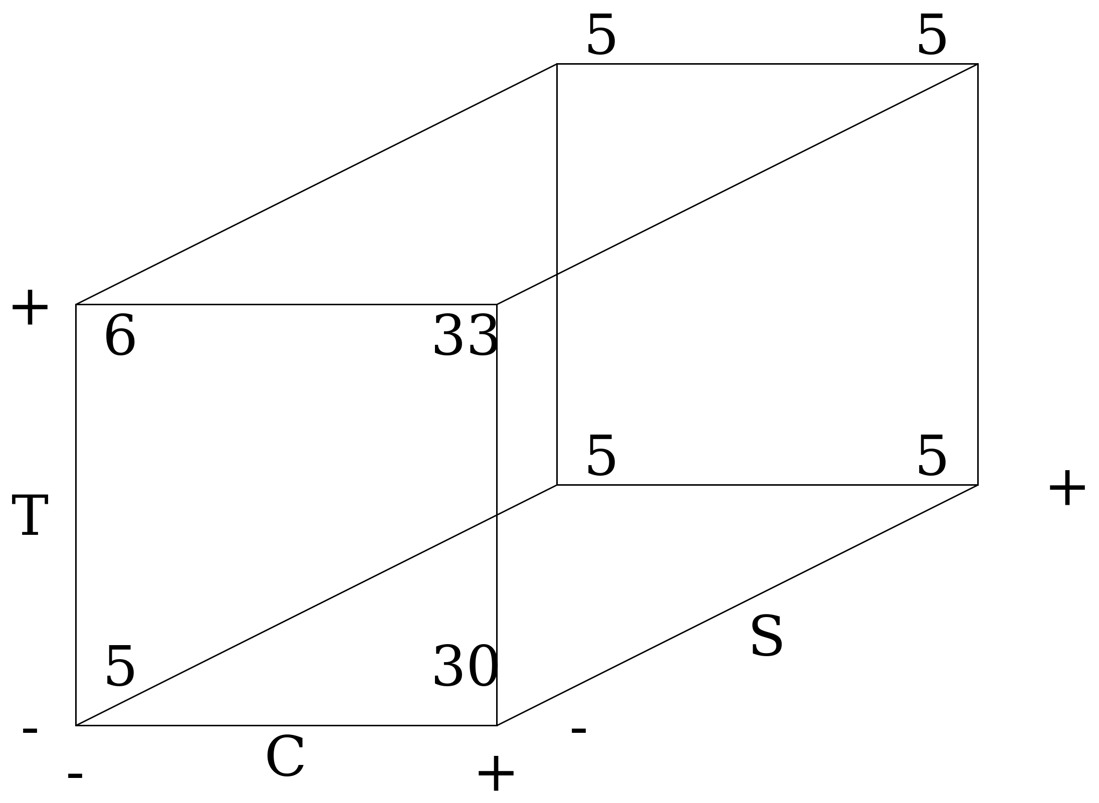
Based on the table of the experiment, we shall make a cube plot (Figure 6).
|
Fig. 6. Cube plot of 3 factors experiment. |
According to acquire results, we need chemical Q with low temperature and hight mixing speed (400 rpm). Let's analyze the main effects and interactions.
Let us start with the first factor C (choice between chemical compounds P and Q, where Q is a high level factor). From the cube plot we can get four estimates of the C effect (along each of the four horizontal edges). At high temperature and high stirring speed (i.e. high T level and high S level) the effect of this factor is 4-5 pounds of contamination. At high temperature and low speed: 33-6. At low temperature and high speed (i.e., T - and S +), the effect is equal: 3 and 4. And finally, at low temperature and low speed: 30 and 5.
We can analyze the obtained information in terms of each factor and their possible interaction.
-
During the tests, the chemical compound showed four results. The average for these four numbers is \(\frac{50}{4} = 12.5\). But what does the resulting number 12.5 really mean? How would you explain this value to your manager, who knows nothing about statistics and experiments?
-
The value of 12.5 indicates that on average we expect to see an increase of 12.5 pounds per ton of pollution when moving from chemical compound P to Q (although the model uses a 6.25 - half coefficient). Therefore, for the features in the model, we write half of the effect (taking into account normalization).
-
The difference between the effects of a chemical at high and low mixing levels (S) is another thing to pay attention to. Note the huge difference, which indicates that there is a clear interaction between factor C and factor S.
-
-
Before we move on to the interactions, let us look at temperature (T). According to the table, there is no noticeable effect of temperature on the system response. This is also confirmed by the calculated coefficient in the model = 1.5 units (or 0.75 when normalizing the effect). This is a really weak effect.
-
Finally, let us consider the effect of stirring speed (S). The average for the effect is -14.5 (or -7.25 when normalizing). In other words, we expect a mean reduction of 14.5 pounds of pollution when moving from low to high mixing speed.
At this stage you should always take a moment to ensure that your results make sense. We can see that switching from chemical P to Q increases contamination (horizontal axis Figure 6). So the value of 6.25 looks adequate. A small value of 0.75 for temperature also looks logical, because it really has a very weak effect. Finally, an increase in stirring speed leads to the most significant reduction in pollution by 7.25 units.
Since we have finished interpreting the individual factors, we can move on to the interactions. Previously, we noted that the effect of the chemical changes greatly when the stirring speed is low. However, on the back edge of the cube (at high stirring speeds) the effect of chemical selection is almost equal to zero. It is obvious that the stirring speed changes the effect of the chemical compound. Thus, we observe the interaction between 2 factors (S and C). For numerical estimation, we will use a familiar technique of adding a new term to the equation.
We have two possibilities to calculate it using different levels of the variable: 1. at high temperature; 2. at low temperature.
We have two possibilities to calculate it using different levels of the variable: 1. at high temperature; 2. at low temperature.
There is no guarantee that the effect will be symmetrical, so we will perform both calculations, and then take the average (even if the effect is symmetrical we will not lose anything, otherwise we will take into account both effects). Next, we normalize it by the number of attribute levels, as always (write half).
So far, we have only considered the interaction between C-S factors. There if no strong interaction for other factors (the low temperature effect is possibilities of it). In fact, there is also a three-factor interaction C-T-S. But it is difficult to calculate it with bare hands. Further on, we will use a computer for this purpose. So let's stop at the results we've got and analyze them for now.
General analysis of results. The main conclusion is that at low mixing speeds chemical Q is not effective, but at high mixing speeds both chemical compounds are equally effective. From this moment, the experiments become a really powerful tool. We saw the lowest level of contamination when using chemical Q with high S and low T (find this value in the cubic diagram). But what if, according to the government, the pollution should be less than 10? And with that, let's say, chemical Q is twice as expensive as P...
In fact, we have now thought about the additional result - profit. Do not forget, that profit (or expenses) often play an important role in all systems. So you should always keep in mind the economic component of each corner of the cube.
At the same time, we have seen a small temperature effect. And here is the question: does it mean that there is no reason to consider temperature as a factor? And the answer is no. It is important to understand, that even minor effects provide us important information about system. So, in our example, we see that in the temperature range \([70; 100]^o F\) temperature has a negligible effect on the amount of pollutants. And this is important, because based on this information, an engineer or operator can choose the most economical working conditions. And again, it all comes down to profit. It's very likely that working at lower temperatures will save energy. And since temperature has only a small impact on the system, we will not have a significant impact on the level of pollution if we decide to work at a lower temperature. And that's a great result.
The challenge. Build a forecast for any case using the cube plot and check it for the model without influences. In which direction do the interactions work (increase or decrease the amount of pollutants)?
The challenge. Why do you think chemical compound Q is less effective at low mixing speed, but works very well at high speed?
2.6 Least square method for two factor experiment model
Coming to this section, we looked at some important examples of how to build and analyze an experiment. Moreover, we learned how to calculate models, which allows us to associate encoded factors with a target variable (output). However, we have chosen coefficients for the model intuitively, based on quite logical assumptions about averaging the effects of features. It is time to describe the model in a more formal way.
To build a mathematically justified predictive model, we will use the most common approach - the method of least squares (LSM). We will discuss the statistical basis of this method in Chapter 3, but for now we will focus on its general features and experimental application. As an example, we will consider our "popcorn experiment". Let me remind you that the linear model for a two-factor experiment generally looks like this:
where \(x_A\) and \(x_B\) are coded factors (features with -1 or +1 values for time (A) and corn type (B)).
We carried out 4 experiments and for each of them our model shall be work. Then:
Therefore, after carrying out the experiment we have 4 equations with 4 unknowns, which means - we can solve them! These equations are linear, so the system of equations is quite simply solved using matrix methods. There is no need to be afraid, it is just a more convenient form of recording and calculation equations. Let me show you how to do it.
In the matrix form, our equations are written down as follows:
Matrix values \(4 \times 4\) consist of coded variables. The other 2 vectors (matrices with one column or row of data) consist of experiment results and unknown coefficients before the coded variables. In the so-called "analytical" form (i.e. which has a strict mathematical justification) such matrix system has a solution:
where \(b\) and \(y\) are vector with unknown coefficients and vector with tests results. The \(X\) is matrix with coded factors.
Note. Factors should not always be coded (normal, "real" values can also be used). However, then we may face a number of problems (unbalanced values, solution instability, etc.). So it is better to always use encoded values (or at least normalized for mean and variance).
It is also possible to find the described solution of matrix equation manually (if the rules of linear algebra are used). However, it is better to use computer programs that will solve these equations very effectively for you. All we need is a \(X\) matrix and a \(y\) vector. And we have everything we need: the \(X\) matrix is the result of the experiment table, and the \(y\) vector is the results of four tests.
For computer calculations, we can use a number of programs. For me, the main ones are: MS Exel, R and Python. As you can see, 2 of the 3 listed programs are programming languages. But you should not fear them. For example, R is a very common and simple language for statistics and data analysis. It is rather easy to install and use while the result is clear. On the other hand, modern Exel provides a very wide range of functions to work with data (including working with models and databases, pivot tables, etc.). In addition, there are many paid and free programs for experiment planning and data analysis. You can search them in the Internet. But in our short course we will consider quite simple examples on R. Besides, you can study R in more detail in this course or this one in Russ..
2.7 RStudio for analyzing results of factors experiments
On the previous examples, you have learned to perform the necessary calculations and analysis of the experiment results by hand. However, using such approach our capabilities are very limited, and the risk of error is very high. It is time to switch to digital technologies. To do this, you will need to choose software to design the experiment and analyze the data. And in my opinion, the R programming language and RStudio programming environment are perfect for it.
R language and software to work with it are free, have an intuitive interface, but most importantly - R is widely used by various companies and researchers. R is so flexible, that you can even use it in a browser. You can take advantage of this feature if you don't want to install software or cannot do it (for example, while using a work computer). However, if you are serious and want to work on your computer, you will need to download two programs: R itself and RStudio. In the first case, you will need to choose the fastest or closest download location (Russia or Germany in my case). Install both software packages on your computer and run RStudio (it will launch R in the background).
Create a new R-script from the "File" menu. In the opened window, we will write our simple commands and design the experiments.
I want to highlight follows:
- first of all, users are often mistaken, because commands in R are case-sensitive (e.g. command
c(1, 2, 3, 4)will create a list with 4 entries, but if you use capitalC(1, 2, 3, 4), nothing will work); - secondly, if you need help, use
help()command.
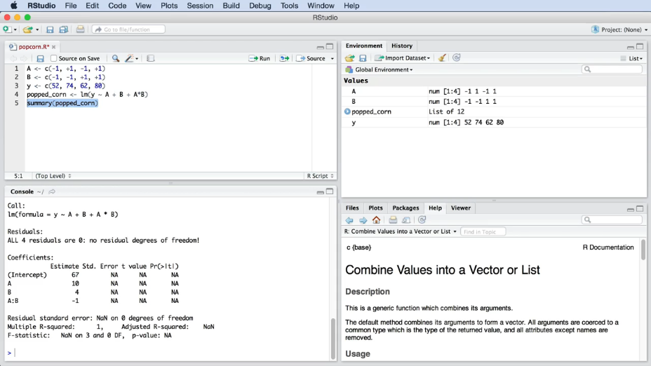
For example, our "popcorn-experiment" and work areas in RStudio are shown on Figure 7.
|
Fig. 7. "Popcorn-experiment" in RStudio. Windows are (from lest to right and upside down): window for script, variables in computer memory, console with results, help windows. |
In the future, instead of screenshots, we will use just code that you can copy and execute in your RStudio:
A <- c(-1, +1, -1, +1)
B <- c(-1, -1, +1, +1)
y <- c(52, 74, 62, 80)
popped_corn <- lm(y ~ A + B + A*B)
popped_corn
Attentive students could notice that the recording of the experiment in the picture and in the code is different and we will soon find out why.
We will start at the end. Variable popped_corn contains the calculated coefficients of the model and simply outputs them to the console (this is the meaning of variables, they are references to certain values or operations, which we have assigned to them). Above, we declare the predicted model, which is called popped_corn. If this is your first time with R, you may be a little scared - I encourage you to be brave and believe in your abilities!
Let's take a look at everything one by one. Let's start with the reverse arrow (<-). It is symbols less (<) and dashes (-), which together look like an arrow. In the R language, this is the assign operation (i.e., we pass a value to a variable and then we can just write a variable to use that value). In other words, we create a variable with the name popped_corn and everything to the right of the arrow are assigned to it (the results of the linear model calculation). lm to the right of the arrow means "linear model" and indicate that we want to use least square methods to build a line. Finally, the tilde symbol (~) in the middle is interpreted as "predicted ..." or "described ...".
Note.
<-and=symbols are almost equivalent in R. However, I recommend to use<-as an assignment operation to avoid confusion. For more information, please read here.
Select all the commands and press Run to run the code. Alternatively, press the Source button (in the modification Source with Echo) without code selection. If we do not get an error message in Console, you will see the result (also in the console) and the existing variables (Environment tab). The output of this small code shows the coefficients for the constructed linear model. We got the 67 for intercept; 10 for the main effect of A; 4 for B and 1 for the two-factor interaction AB. Note, that these numbers exactly match our manual calculations.
This is the whole programming magic. It is really the fastest and most convenient way to get a model with computer help.
Note. The formula that describes the linear model has values for A, for B and for the AB interaction. But there is no variable for intercept (constants). R creates it automatically and when you enter only three parameters, R will show you four.
In Figure 7 you can see the command summary(popped_corn) instead of just calling popped_corn. This command provides you more statistical data for calculated parameters: coefficient errors, average square deviation, etc.. We will learn more about these parameters in 2 and 3 parts of our course.
Note. In any calculation program you should get exactly the same parameters for "popcorn-experiment". This is a good check of software and calculation quality.
The challenge. Try to find instructions on the Internet about "how to calculate coefficients using the least squares method in MS Exel". Use "popcorn experiment" data as an example.
Let's continue our introduction to R. The next example is calculation of a three-factor experiment in water purification.
Open RStudio and create a new file for the example of wastewater treatment. It is very useful to specify our model at once and then declare all necessary variables.
water <- lm(y ~ C + T + S + C*T + C*S + S*T + C*T*S)
Remember that in the example of water treatment we considered three factors: C (chemical), T (temperature) and S (mixing speed). We also have three two factor interactions (CT, CS and ST) and one three factor interaction (CT*S). At the same time, we have the results of eight experiments.
Note. When conducting an experiment and analyzing the results, keep in mind that we will always need to conduct at least as many experiments as the unknown parameters in our model. For example, the "popcorn-experiment" have 4 parameters (2 single, 1 interaction and 1 intercept point) and 4 experiments. In the example with water treatment we have 8 experiments, so we can estimate 8 parameters (with interaction and intercept).
Notice that we can let R automatically set the encoded values C, T and S using the following code:
C <- T <- S <- c(-1, +1)

design <- expand.grid(C=C, T=T, S=S)
C <- design$C
T <- design$T
S <- design$S

water <- lm(y ~ C + T + S + C*T + C*S + S*T + C*T*S)
Run this code to create a linear model. To output the calculated coefficients to the console, use summary(water) command. Please note that the obtained parameters match our manual calculated values: 11.25, 6.25, 0.75, etc.
Note. We can add a little trick to set our model (this reduces the possibility of error). The results of the model will be similar (please check).
# We use a simplified model mode
water <- lm(y ~ C*T*S)
Note. When planning each experiment, always create a new code yourself. In this way, you will have some "outline" of the work, and it will be especially useful if you use comments (# strings, that are not accepted as code by R). This will solve the frequent problem of losing the results and description of the experiment. For example, you've done the work, and in a few months you need to go back to it and answer your boss' questions or pass the project on to your colleague. If you give them only an Excel file or a set of documents that do not have a step-by-step description, it will be very difficult to reproduce your actions and thoughts. I come across this very often in my practice and urge you to avoid repeating both my and others' mistakes!
Writing well commented and consistent code creates a well tracked and reproducible record of your work. This is a very important criterion for many companies and laboratories (some even have special requirements for traceability of work, for example ISO 9001-2015).
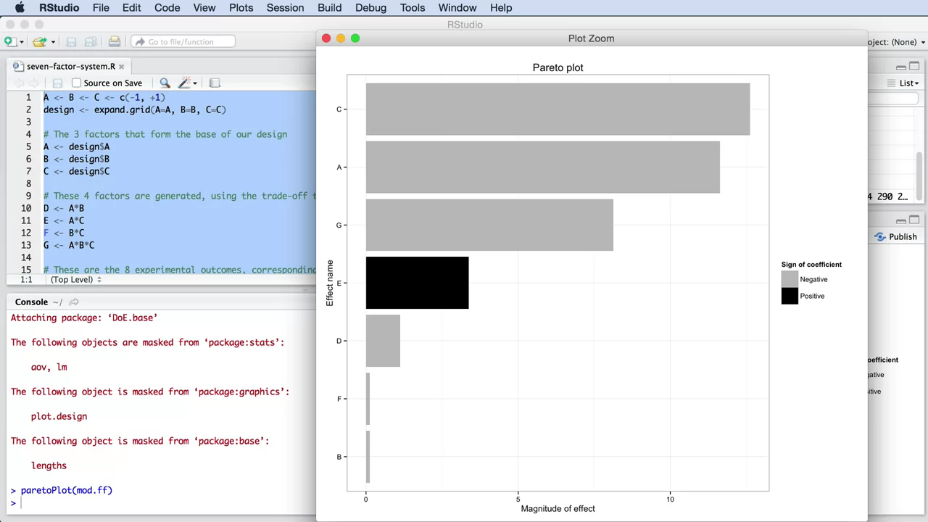
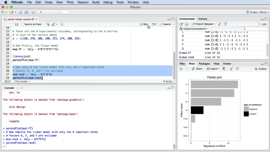
Here is one more code fragment that will help us interpret the results of the experiment. It allows us to visualize the influence of each effects within the obtained model (the greater is the absolute value of a parameter, the greater is its influence).
# Estimation of factor influence. Firstly, setup "pid" package: Tools -> Install Packages -> pid
library(pid)
paretoPlot(water)
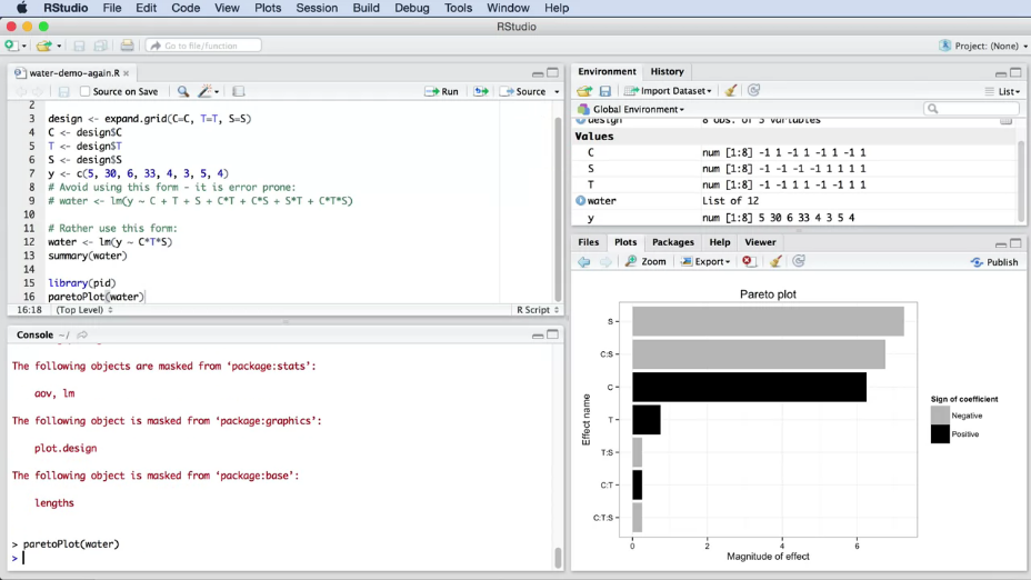
The result is shown on Figure 8.
|
Fig. 8. Example of factor comparison, using the Pareto plot in RStudio. |
The histogram shows the absolute value of each of the model parameters (this allows to estimate the scale of influence of each of the coded features). The parameters sign is also important, it shows the directions of the factor's influence. But for better visual comparison it is more correct to use absolute values (the sign is highlighted in a different color). Such diagrams are often used to identify variables, that are not relevant for model and can be removed from the model. A histogram shows sorted values from the highest to the lowest absolute value. This allows us to quickly find the most important factors of the system. The longest bars correspond to the factors that most significantly affect the result.
Note. It is often important to use a clear black and white comparison, as not all people distinguish colors. In addition, sometimes it is necessary to print the report on a black and white printer.
Let's analyze the plot. You will immediately notice that the \(C \times T \times S\), \(C \times T\) and \(T \times S\) interactions are small, when compared to other parameters. The most significant factor is S. The color of the band indicates that S has a negative effect on the result. As you will remember, our goal was to minimize the pollution, so we immediately realize that increasing S will reduce the pollution, which is good. Another important factor is the effect of the chemical, C. Its effect is positive, i.e. if we choose the positive coded value of this categorical feature, we will get an increase in pollution.
Let us consider an even more complicated example - a four factor experiment with 2 measured parameters. This is a good problem from Box, Hunter and Hunter's textbook. In this experiment, we use solar collectors and heat accumulators. Values of result of experiment are received from computer simulation (see the site).
Note. A little advice related to the simulations. Usually it is very simple to perform a simulation and there is a temptation to investigate it ineffectively. Often you will meet people who just play with the software by entering different values until they get the right answer. But the simulation should be taken as seriously as the real model. Always use a systematic approach and conduct factor experiments on it.
Note. There are two key advantages to using computer simulations: * fast results with sufficient computational power of the computer (or running in parallel mode); * it is possible to not randomize the order of experiments. The reason for this is quite simple - there are usually no random and systematic errors in the simulations, which depend on the time and external parameters of the experiment. When you repeat the simulation by entering the same initial values, usually you get the same answer. But be careful: some computer experiments do not give identical results when you repeat them, and in any case it is better to always use a random order. The cost of doing this is minimal, but it will protect you from a number of problems.
So, back to the solar water heater. We're looking at four factors: * A - the amount of sunlight (insolation); * B - heat storage capacity (tank volume); * C - the water flow through the absorber; * D - interruption of sunlight (cloudiness).
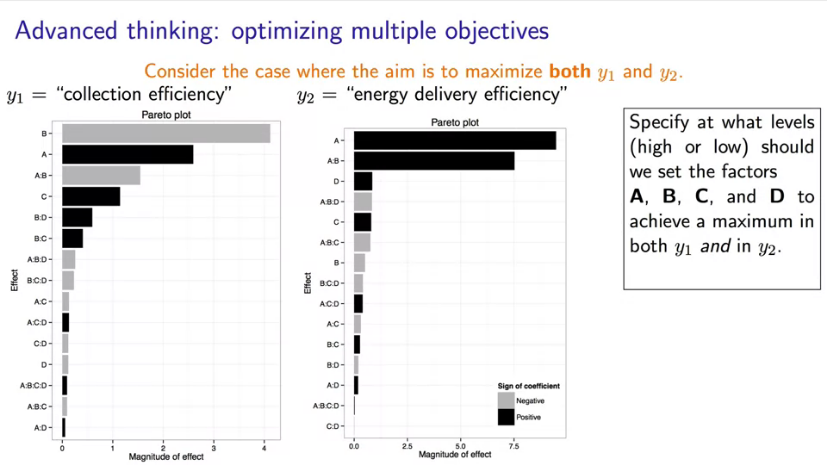
In terms of the influence of these factors, two outputs are considered: * \(y_1\) - energy collection efficiency; * \(y_2\) - energy transfer efficiency.
You can immediately determine how many experiments will be conducted. It is \(2^4 = 16\) tests if each factor has two levels (low and high).
So, there have been 16 tests and it is time to make up the code for model calculation:
# Solar panel case study, from BHH2, p 230
# ----------------------------------------
A <- B <- C <- D <- c(-1, +1)
design <- expand.grid(A=A, B=B, C=C, D=D)
A <- design$A
B <- design$B
C <- design$C
D <- design$D

# y1 - collection efficiently
y1 <- c(43.5, 51.3, 35.0, 38.4, 44.9, 52.4, 39.7, 41.3, 41.3, 50.2, 37.5, 39.2, 43.0, 51.9, 39.9, 41.6)

# y2 - energy delivery efficiency
y2 <- c(82, 83.7, 61.7, 100, 82.1, 84.1, 67.7, 100, 82, 86.3, 66, 100, 82.2, 89.8, 68.6, 100)

model.y1 <- lm(y1 ~ A*B*C*D)
summary(model.y1)
paretoPlot(model.y1)

model.y2 <- lm(y2 ~ A*B*C*D)
summary(model.y2)
paretoPlot(model.y2)
Note. The reason why the \(A \times B \times C \times D\) record works is because of the model hierarchy principle for R. Let's look at a simple example. If you wrote only \(A \times B\), R will automatically include factor A and factor B in the model. After all, there can be no two-factor interaction of \(A \times B\) if there is no factor A and factor B.
After the code is executed, you should study the obtained results. For this purpose, let's build two separate linear models and Pareto diagrams (Figure 9): for the efficiency of energy collection y1 and for the efficiency of energy transfer y2.
|
Fig. 9. Example for factor importance calculate with Pareto plots. |
As you remember, gray bars indicate a negative factor influence on the output, and black bars indicate a positive factor influence. According to the obtained model for energy collection efficiency (\(y_1\)) the biggest influence belongs to factors B and A, interaction \(A \times B\) and factor C. Other interactions have a lower impact on the result.
- We can observe a decrease in system response when factor B increases. In other words, when the tank volume increases, the collection efficiency decreases. This is the most important variable in the system.
- Further, factor A (amount of sunlight) has a positive effect on the collection efficiency.
- What kind of interaction do you think \(A \times B\) will have? The correct answer is a high level for factor A and a low level for factor B. We can see it from the equation and the Pareto diagram. In this case, result increase from factor B and simultaneously makes the two-factor interaction work for us.
- factor D has little effect on the result. This is a useful conclusion because it shows that cloud didn't bother us. If we had to do more experiments in the future, we could no longer include factor D.
Thus, A, B and interaction A*B are the three most influential parameters of the model. Try to explain the influence of other factors by yourself.
Now let's look at the second output variable - energy transfer efficiency \(y_2\). If you study the corresponding Pareto diagram, you will see the following.
- Huge influence of factor A.
- Big influence of two-factor interaction \(A \times B\).
- Influence of C and D factors is insignificant.
The explanation is yours.
Note. You may have noticed that many high-level interactions (three-, four-factor and more) are small or equal to zero. This happens quite often and we will see how this can be used.
Note. I would like to mention an important thing on the analyzed data. In case of the \(y_2\) model, the influence of factor B is small and you can conclude that factor B is not important. But this is not quite true. We cannot exclude factor B from the model because the \(A \times B\) interaction is very important. This means that the influence of factor A depends on the level of factor B and vice versa. Therefore, we cannot ignore factor B.
Considering such an example, we come to the key question of experiment planning: can we simultaneously optimize both \(y_1\) and \(y_2\)? What would be the best combination of factor levels that gives this maximum?
2.8 Reduce experiments expenses
Before answering the question about the model variable optimization, you should understand how to optimize the cost factor.
As you can see, the number of experiments (and thus time and cost) increases in degree depending on the number of factors. Let's try to get rid of this limitation.
So far, we have considered so-called full-scale experiments, when the influence of each factor was fully studied for the model creation. In other words, we studied every change in every factor. But how can we reduce the number of experiments? This is possible by using half, quadro and etc. (by 2 times) experiment scheme. For example, using half-factor experiments involves cutting the number of experiments by half.
Of course, everything has a price and such actions will lead to information reduction. But there are 2 significant reasons for that:
- The cost of each experiment can be high.
- There is no confidence in the obtained results. What factors will be significant? Will the obtained data be optimal, etc.?
According to the famous scientist George Box ** for the first experiments and works should be allocated about 25 \% of the total budget and no more**. We will need the rest in the further research process. Therefore, we need to understand that our initial assumptions are not absolute and may be quite wrong. This means we need insurance and the possibility of additional experiments.
Let's study what result will we have in half-factor experiment and how to do such tests.
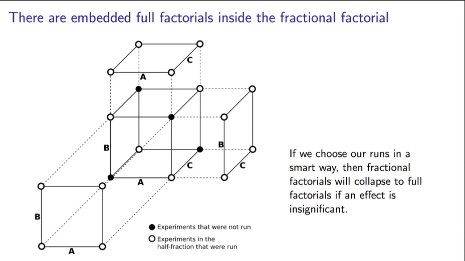
There is special scheme for choosing meaningful tests from our ideal full-factor experiment: open or closed loop selection. Let's consider a familiar example of water treatment in terms of half-factor experiments (Figure 10).
|
Fig. 10. Selection of meaningful combination of factors for half-factor experiment. |
Note. Feature values have changed to A, B, C for better convenience.
Note that this choice of experiments implies a complete change of factors A and B, while factor C is chosen as a result of the multiplication of the first encoded factors (keeping the sign as in Figure 10).
This approach to the experiment allows us to win jackpot if one of the factors turns out to be unimportant for the model. Then one of the directions of the cube will disappear and we will reduce the necessary number of experiments by half, and with earlier carried out tests we will have a full-factor experiment... Profit!
But that's only one side of the coin. Let's see what model we can get if we do a half-factor experiment:
# Half-factor experiment
# ----------------------------------------
# full-factors for A and B
A <- c(+1, -1, -1, +1)
B <- c(-1, +1, -1, +1)
# C = AB
C <- c(-1, -1, +1, +1)

# y - purify efficiently
y1 <- c(30, 6, 4, 4)

water <- lm(y1 ~ A*B*C)
summary(water)
You can see a lot of NA (not applicable) for interaction coefficients and these are normal. The model doesn't have enough data. But we don't need these factors. Let's compare the resulting equation to the original one:
We have very similar coefficients (3 from 4 are very close to each other)! In other hand, the B coefficient is wrong and we don't have the factors interaction.
Let's take a closer look at what happens in a half-factorial experiment.
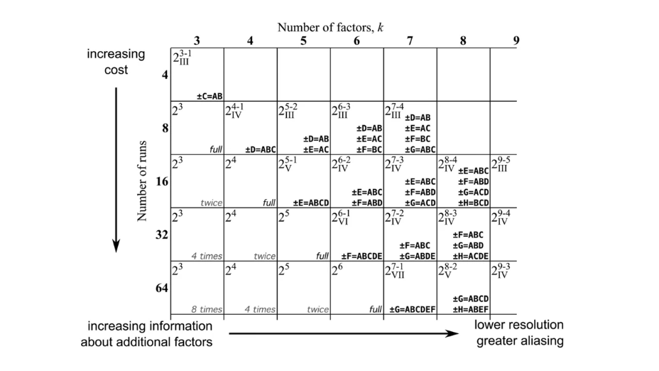
We have already described the logic of choosing necessary combinations of factors. However, we can get a generalized view of the selection of factors for half-factor and other type of experiments from a special table (trade-of-table, Figure 11).
|
Fig. 11. Trade-of-table for experiment schemes. |
Or you can use R:
library(pid)
help(tradeOffTable)
Further on, we will return to studying this table, and for now we will look into it to choose how to encode our factors.
The next interesting question is what are the new coefficients and why do they differ from the full-factor experiment? That's the key point to understanding. Actually, the coefficients in a half-factor experiment ** are a combination of elements from a full-factor experiment**. Consider this in the example of water purification.
In a full-factor experiment, we have the following system of equations:
Use only selected features we can write equations as follow:
I pointed out, that these are not mathematical justification, but only the logic of half-factor experiment.
We cannot remove any of the last vectors with coefficients as each of them corresponds to the change of the factor, i.e. the length of matrix X, which remains unchanged. However, such a matrix record of multiplication makes no sense - it is necessary that the matrix dimension of \(X\) corresponds to the dimensions of vectors \(y\) and \(b\). To make the matrix multiplication (and the system of linear equations itself) look correct, it is necessary to reduce the matrix dimension of \(X\). For this purpose, note that the columns of this matrix are actually duplicated. In other words, parts of the coefficients correspond to the same coding of the remaining factors. Behind this lies the same influence of the investigated factors, which we will not be able to distinguish from each other in our experiment (from the mathematical point of view they will be identical).
Thus, if we record a real matrix system for a half-fraction experiment, the obtained coefficients will actually be a linear combination (aliasing, confounding) of the coefficients of a full-factor experiment:
In other words, our new coefficients contain the influence of interaction of these factors besides the influence of "pure" factors A, B, C. This explains that the program outputs us only 4 factors and they differ from the initial factors of a full-factor experiment.
Note. Return to the comparison of the equations of a full-factor experiment and half-factor experiment and make sure that the new coefficients are actually linear combinations of the true ones.
This is how we have reduced the number of factors by eliminating the interaction, but have taken it into account in our new coefficients!
After we have learned about full-factor and half-factor experiments, we can suggest 2 possible goals of the experiment (and ways of its planning):
- scanning (screening) - when we allow reduction of information about the system (for example, do not take into account interactions or get some incorrect parameter estimates) and carry out reduced factor experiments. This is done in order to get a general idea of the interactions in the system.
- optimization - searches for the optimal response value. At such scheme reduction of experiments is not allowed and carrying out of full-factor experiment is required.
Thus, it is always necessary to plan and evaluate the effect of each factor and their interactions (scanning experiments) before optimization experimental work. Here are some useful preliminary conclusions on an example of water purification (a full-factor experiment require 16 very costly tests, and we consider 3 factors: A - temperature, B - mixing speed and C - chemical).
- It is important to code your factors correctly when conducting a half-factor experiment. This will allow to get coefficients that are close to reality. For example, in the above encoding we can conclude that \(\hat{b_C} = b_C + b_{AB} \approx b_C\) because we know, that there is no interaction between mixing and water temperature. In this way, we get a clear understanding of the impact of chemical choice on water purification.
- We should use several encodings and look at the expected results of half-factor experiments. Choose the most interesting ones.
- Always make half-factor experiments first, evaluate the results and only then "finish" the full-factor experiment (if everything is okay and you need more information).
So far, we had considered a lot of experiment and its results. There are a lot of themes, that I want to translate from my course (in Russ.), but it will cost me a lot of time. Further, you find only the table of contents of remain themes and Figures and Tables, which are related to them. If you interested in this course, please contact me via e-mail (or use "Comment" button) and I sent you the material or post it here as fast, as possible.
2.9 Experiment map construction
2.9.1 Disturbances
2.9.2 Blocking the interfering factor in the model calculation
Table 5. Examined factors when introducing an mobile application to the market.
| Low level (-) |
Hight level (+) |
|
|---|---|---|
| A "Promotion" | 1 free-in-app upgrade | 30 days trial of all features |
| B "Message" | "CallApp" has your schedule available at your fingertips, on any device | "CallApp" features are configurable; only pay for the features you want |
| C "Price" | in-app purchase price is 89 $ | in-app purchase price is 99 $ |
Table 6. Blocking of interfering factor, when introducing an mobile application to the market.
| A "Promotion" | B "Message" | C "Price" | D = ABC "OS" | Outcome | |
|---|---|---|---|---|---|
| 1 | - | - | - | - (Android) | y_1* = y_1 + g |
| 2 | + | - | - | + (iOS) | y_2' = y_2 - h |
| 3 | - | + | - | + | y_3* = y_3 - h |
| 4 | + | + | - | - | y_4' = y_4 + g |
| 5 | - | - | + | + | y_5* = y_5 - h |
| 6 | + | - | + | - | y_6' = y_6 + g |
| 7 | - | + | + | - | y_7' = y_7 + g |
| 8 | + | + | + | + | y_8* = y_8 - h |
2.9.3 Analysis of linear combination of factors (aliasing) and planning of scanning experiments
Table 7. Conducting a quarter-factor experiment with an additional test experiment (9th).
| Experiments | A "temperatire" | B "dissolved oxigen" | C "substrate type" | D = AB "agitation rate" | E = AC "pH" |
|---|---|---|---|---|---|
| 1 | - | - | - | + | + |
| 2 | + | - | - | - | - |
| 3 | - | + | - | - | + |
| 4 | + | + | - | + | - |
| 5 | - | - | + | + | - |
| 6 | + | - | + | - | + |
| 7 | - | + | + | - | - |
| 8 | + | + | + | + | + |
| 9 | + | 0 | 0 | 0 | + |
Table 8. Conducting a scanning quarter-factor experiment with an additional test experiment (9th)..
| Experiments | A | B | C | D=AB | E=AC | F=BC | G=ABC | y |
|---|---|---|---|---|---|---|---|---|
| 1 | - | - | - | + | + | + | - | 320 |
| 2 | + | - | - | - | - | + | + | 276 |
| 3 | - | + | - | - | + | - | + | 306 |
| 4 | + | + | - | + | - | - | - | 290 |
| 5 | - | - | + | + | - | - | + | 272 |
| 6 | + | - | + | - | + | - | - | 274 |
| 7 | - | + | + | - | - | + | - | 290 |
| 8 | + | + | + | + | + | + | + | 255 |
|
Fig. 12. Results of conducted experiment. |
|
Fig. 13. The result of the experiment after removing insignificant factors. |
2.9.4 Response Surface Methods (RSM)
|
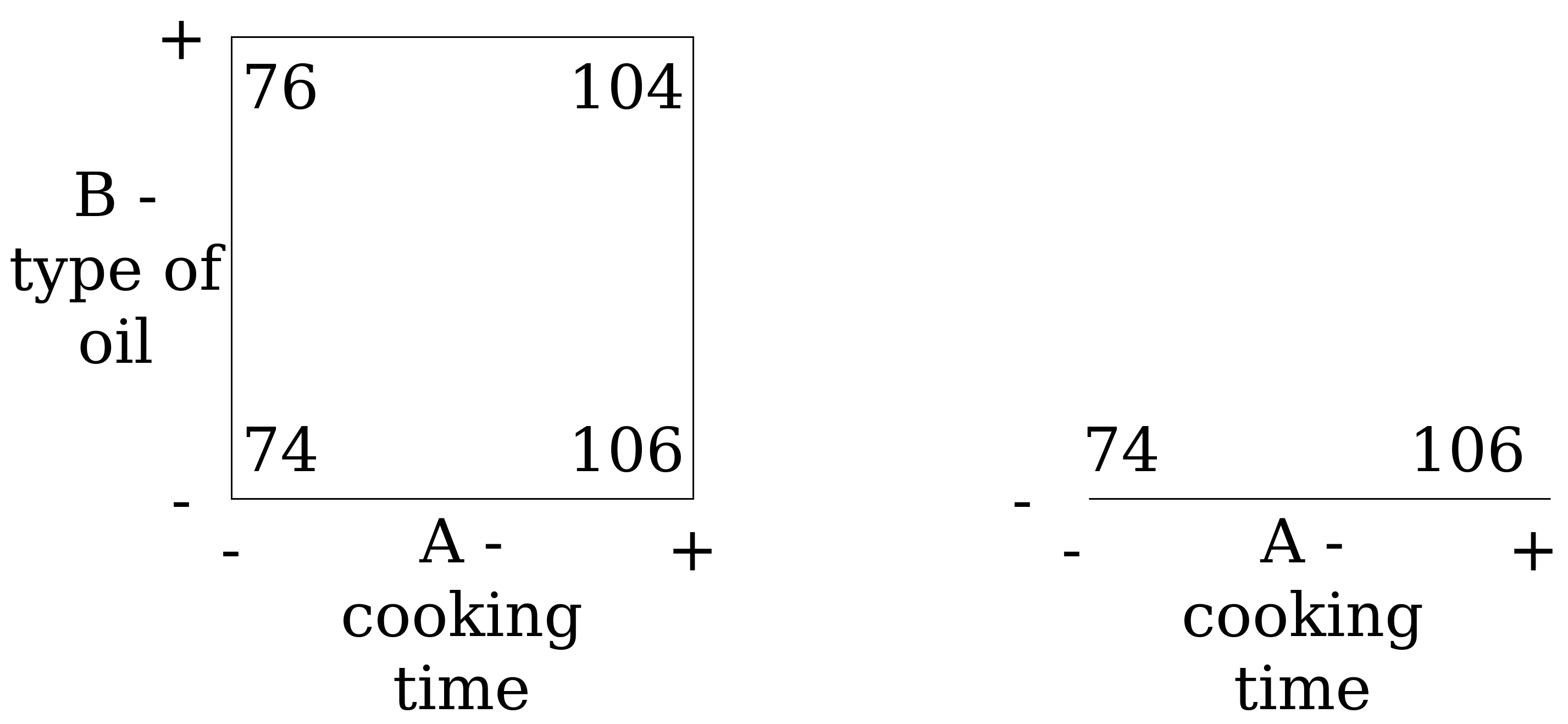
Fig. 14. The result of full-factor "popcorn-experiment". |
|
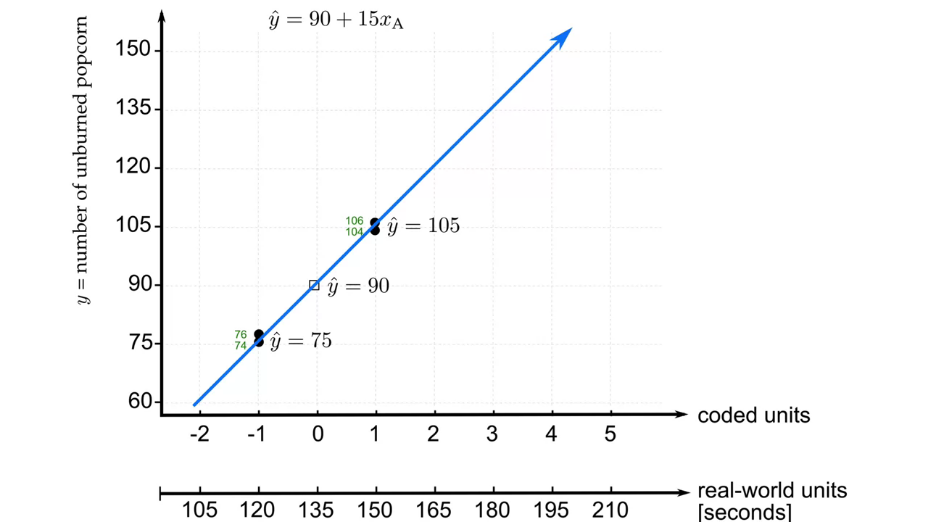
Fig. 15. Obtained model for one-factor "popcorn experiment". |
|
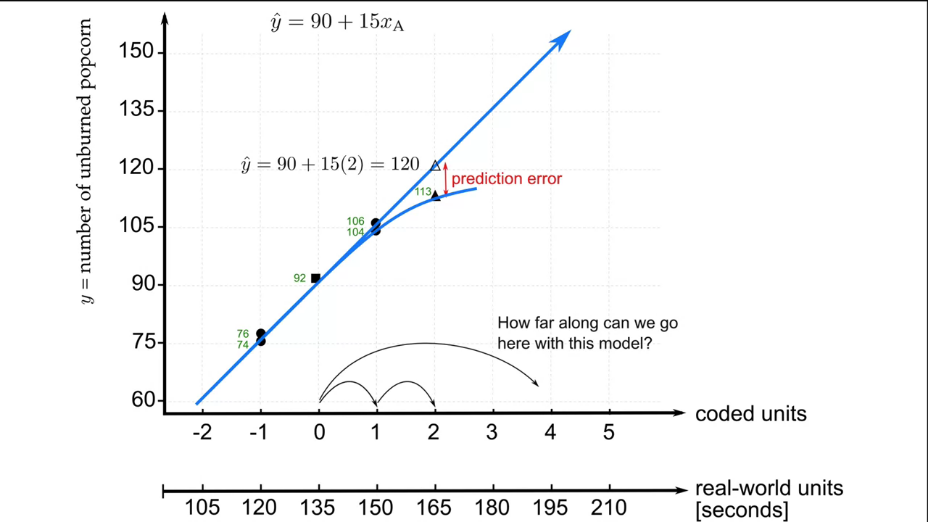
Fig. 16. Next experiment outside the model definition area. Evaluation of usability. |
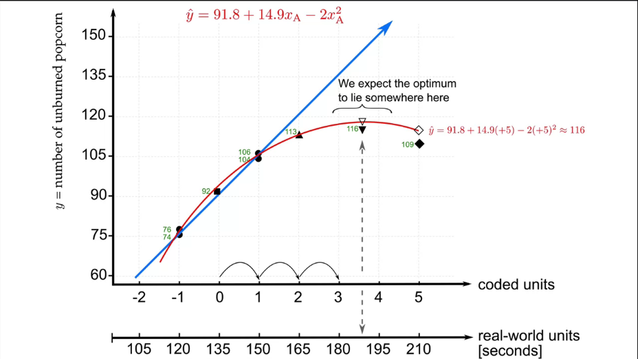
|
Fig. 17. Complication of the model. |
2.9.5 Response Surface Methods (RSM). Complication of the model.
|
Fig. 18. Optimization surface and contour lines. |
|
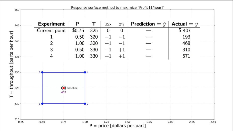
Fig. 19. Initial full-factor experiment. |
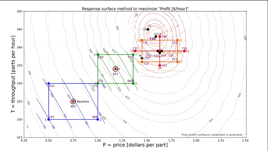
|
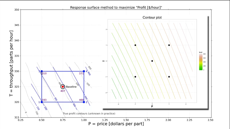
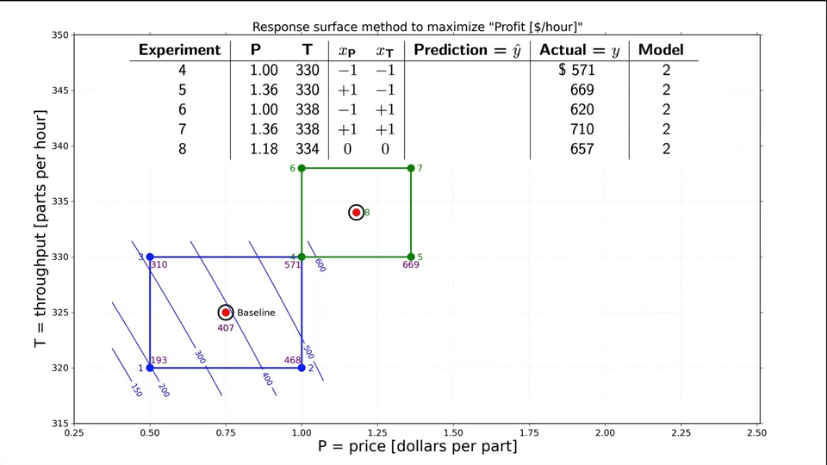
Fig. 20. A response surface methods (RSM) to maximize production profits. Comparison of contour lines. |
|
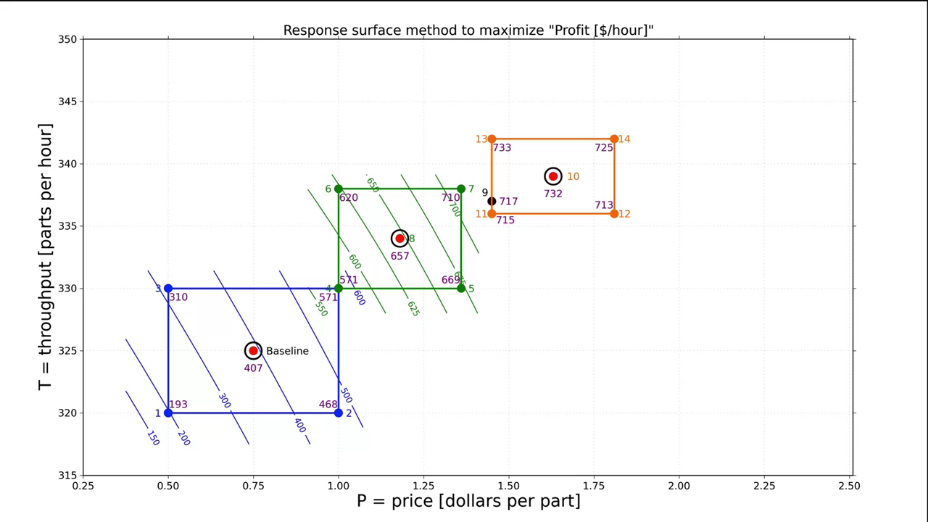
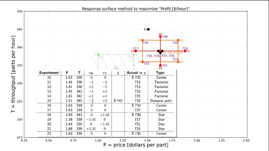
Fig. 21. A response surface methods (RSM) to maximize production profits. The next factors experiment. |
|
Fig. 22. A response surface methods (RSM) to maximize production profits. The next factors experiment. |
|
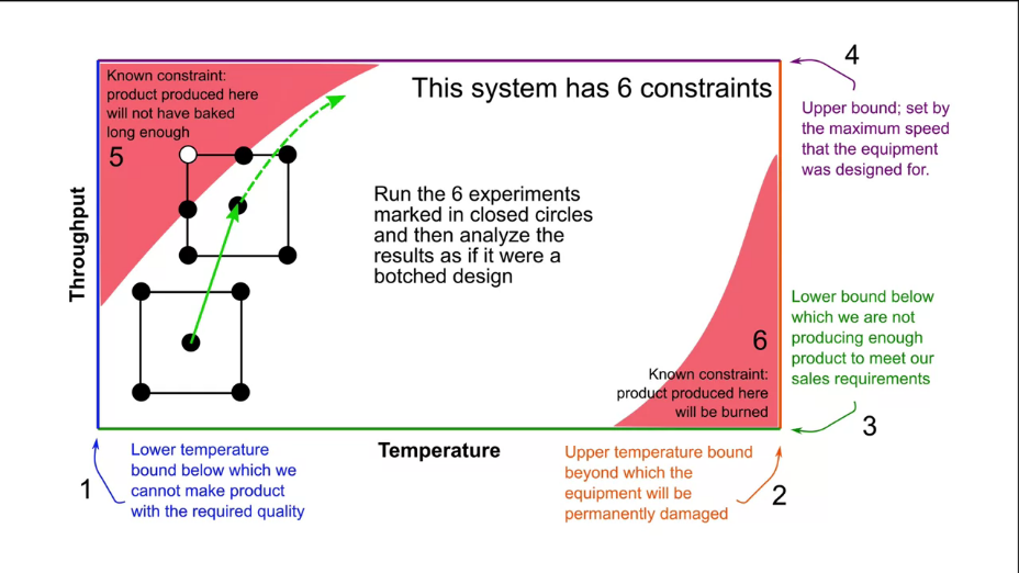
Fig. 23. An example of limitations in a system that provide asymmetry. |
|
Fig. 24. A response surface methods (RSM) to maximize production profits. The next factors experiment (assume that contour lines are linear). |
|
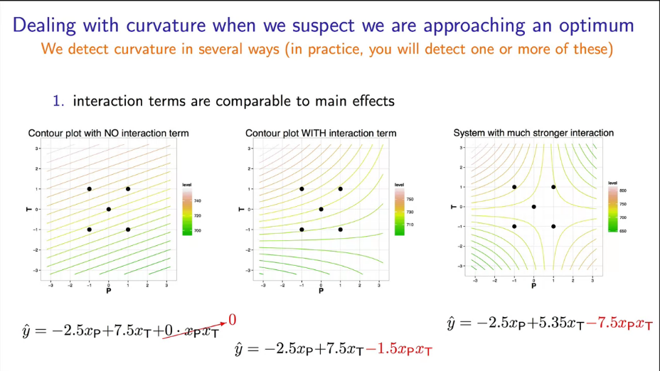
Fig. 25. Type of contour lines depending on the interaction of factors. |
|
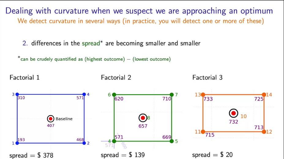
Fig. 26. Spread depending of optimum distance. |
|
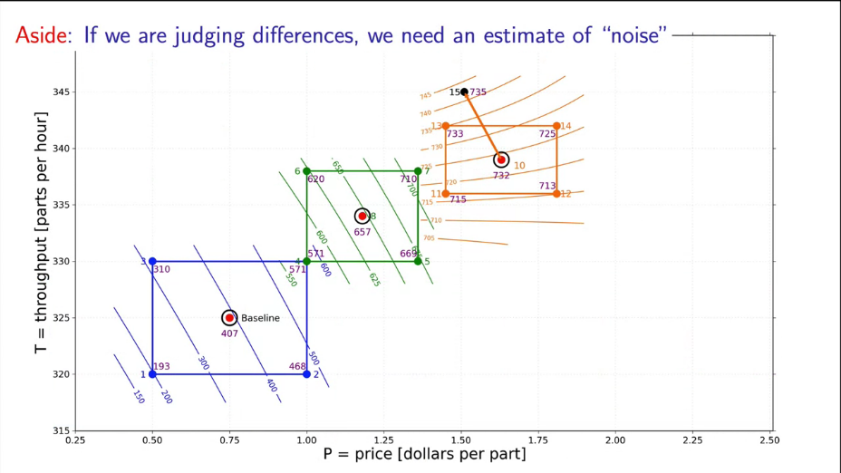
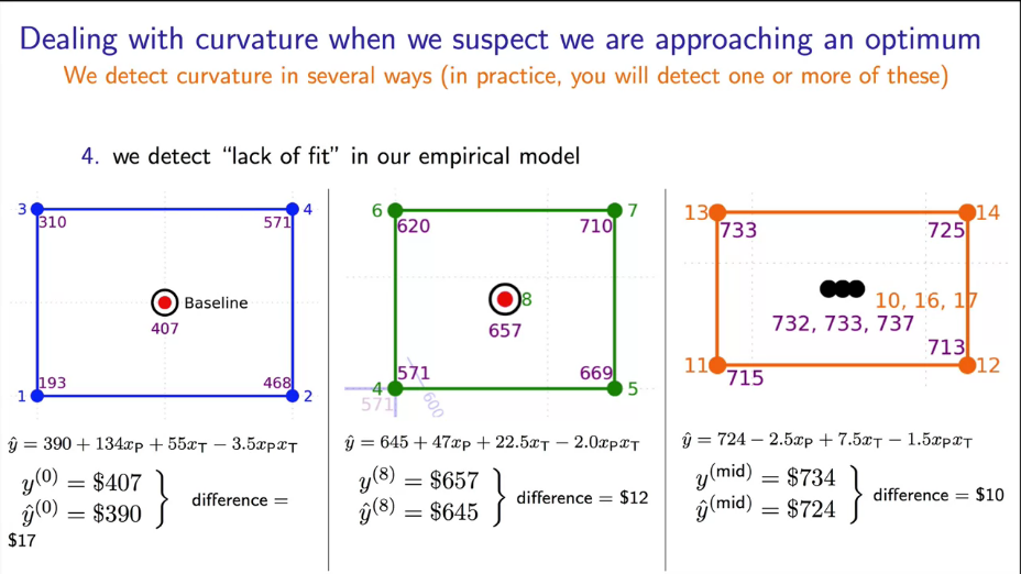
Fig. 27. "Lack of fit" effect. The last full-factor experiment shows 3 additional experiments to determine the noise level. |
|
Fig. 28. Nonlinear model. |
|
Fig. 29. Nonlinear model. Contours lines of optimum (calculated and real). |
2.10 Conclusion
2.11 Questions
3. Comparison experiments. Statistical practice
3.1 Introduction
3.2 Type of representation of sample or general population
|
|
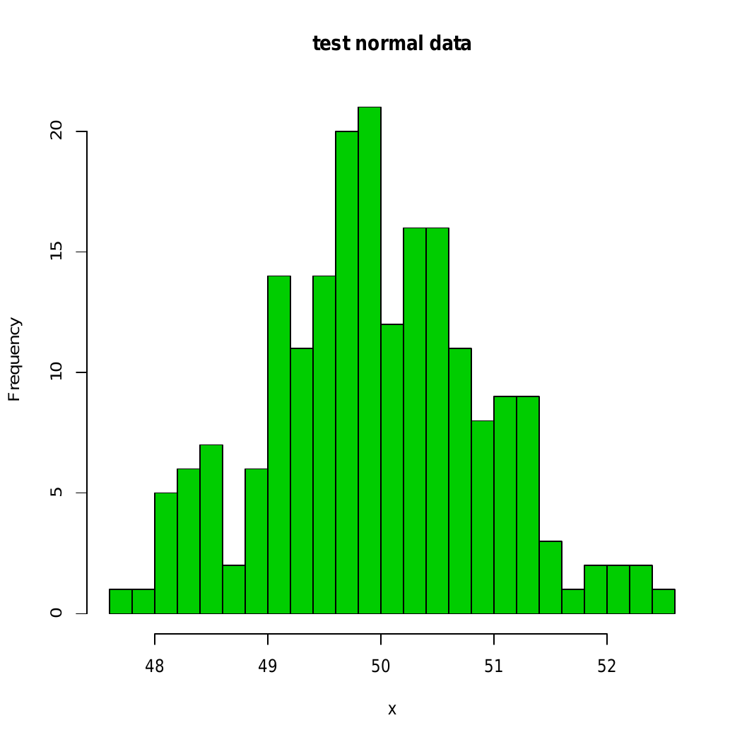
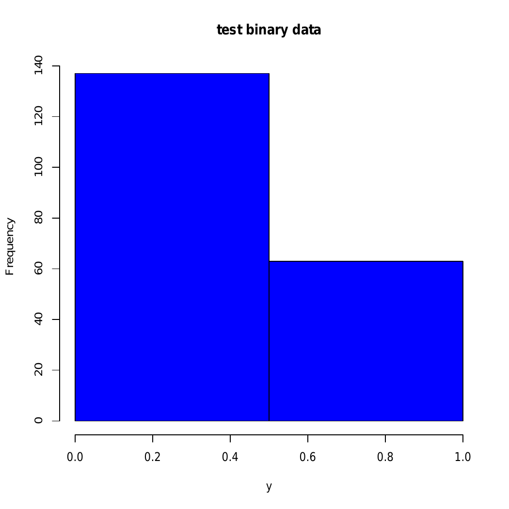
Fig. 30. Histograms for quantitative (numerical) (a) or qualitative (categorical) (b) features. |
3.2.1 Representation of central tendency
div>
|
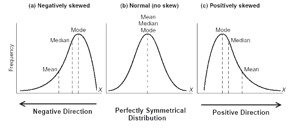
Fig. 31. Example of distributions at different values of mode, median and average (taken from https://stats.stackexchange.com/). |
3.2.2 Representation of variability
3.2.3 Quantiles of distribution
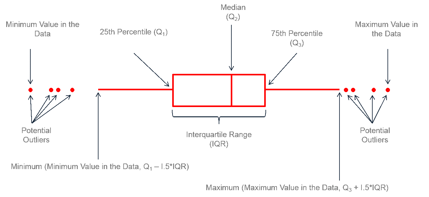
|
Fig. 32 (a). Anatomy of box plot (a). |
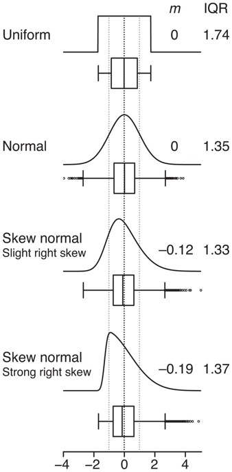
|
Fig. 32 (b). Examples of box plot from https://media.nature.com site and distributions, which are related to them. |
3.3 Statistics and data comparison
3.3.1 Normal distribution
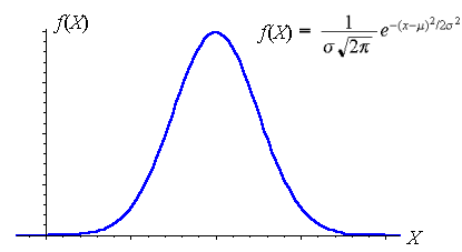
|
Fig. 33. Normal distribution. |
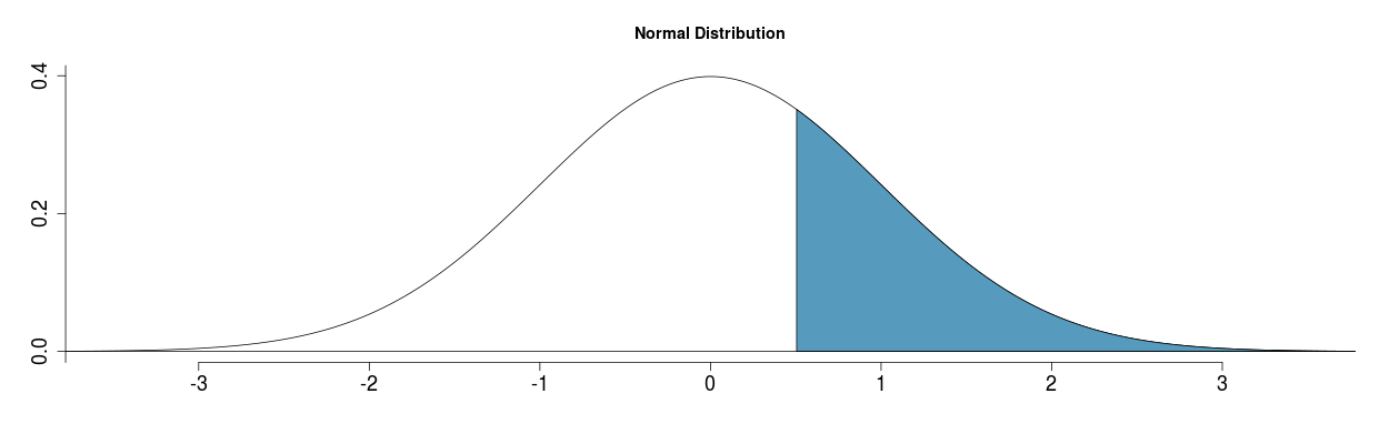
|
Fig. 34. Example for calculating the percentage of observations. |
3.3.2 Central limit theorem
3.3.3 Confidence intervals
3.3.4 The idea of statistical conclusion, p-value of significance
3.3.5 Practice of using statistics to compare data
|
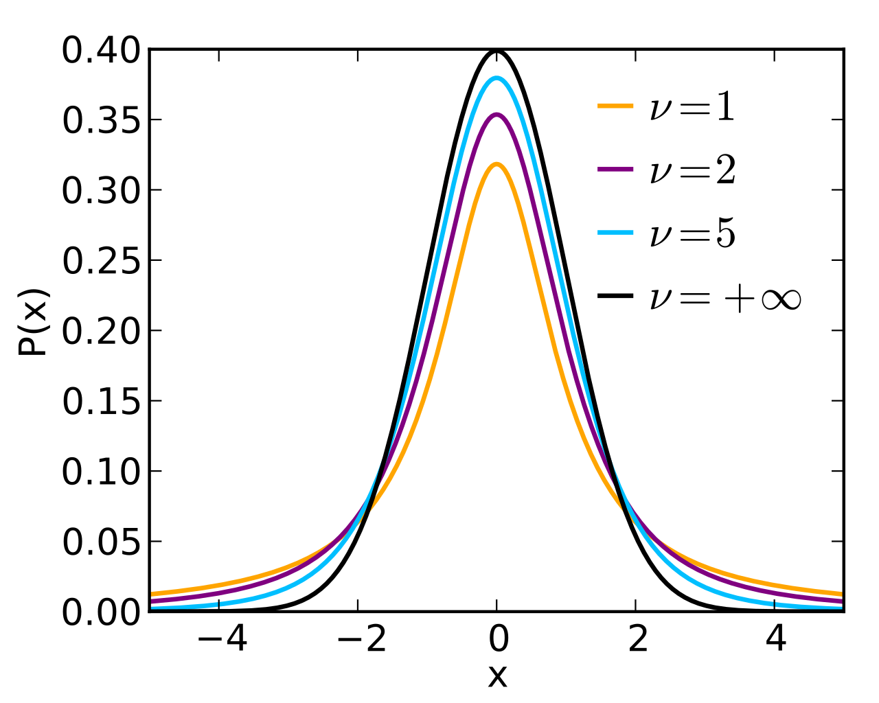
Fig. 35. t-distribution (Student's). |
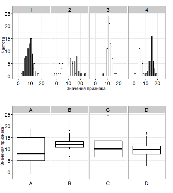
3.3.6 Graphical comparison of distributions
|
Fig. 36. Example of data representation in histogram form. |
|
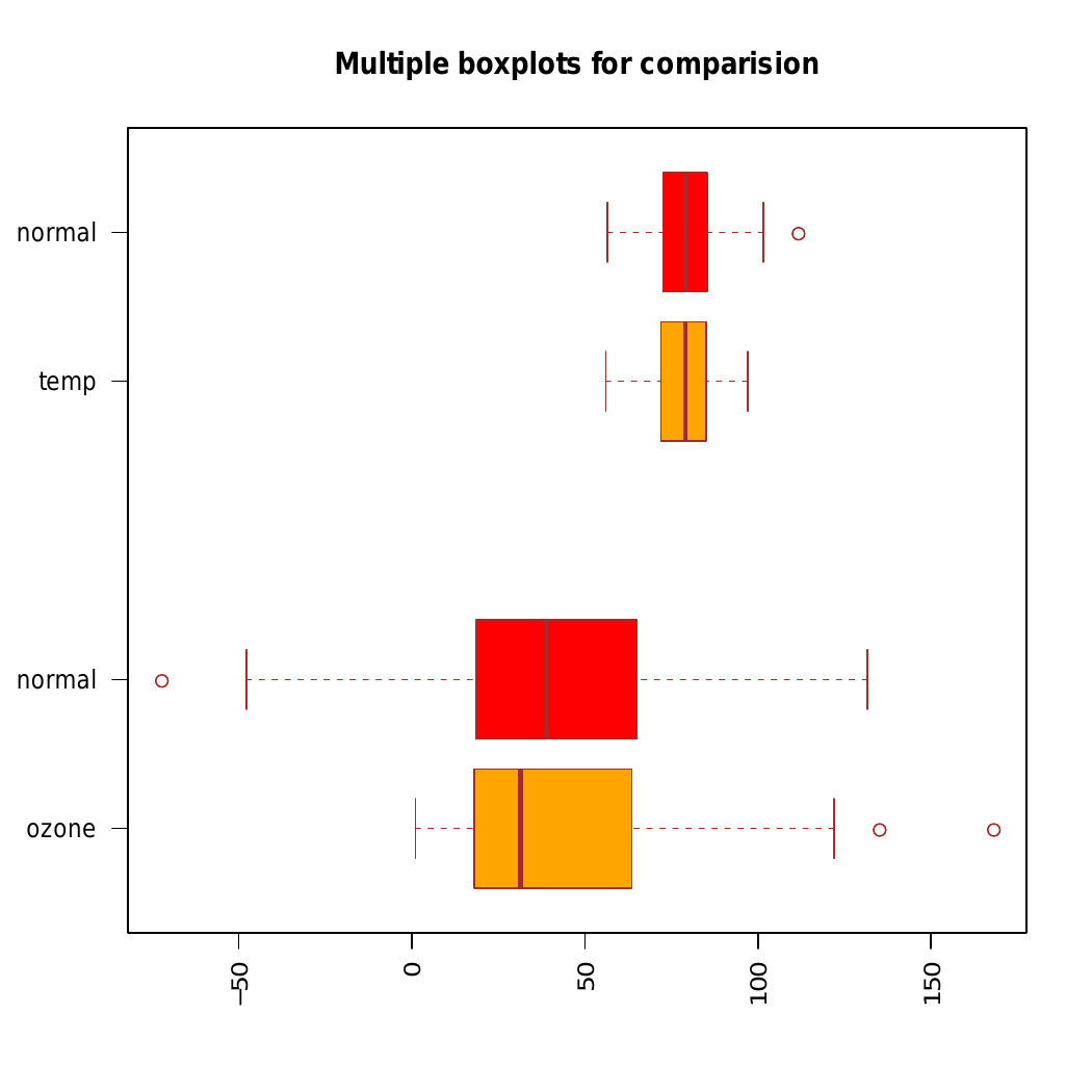
Fig. 37. Example of data representation as box plot. |
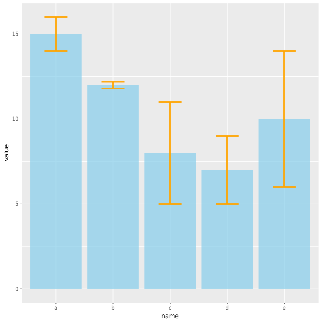
|
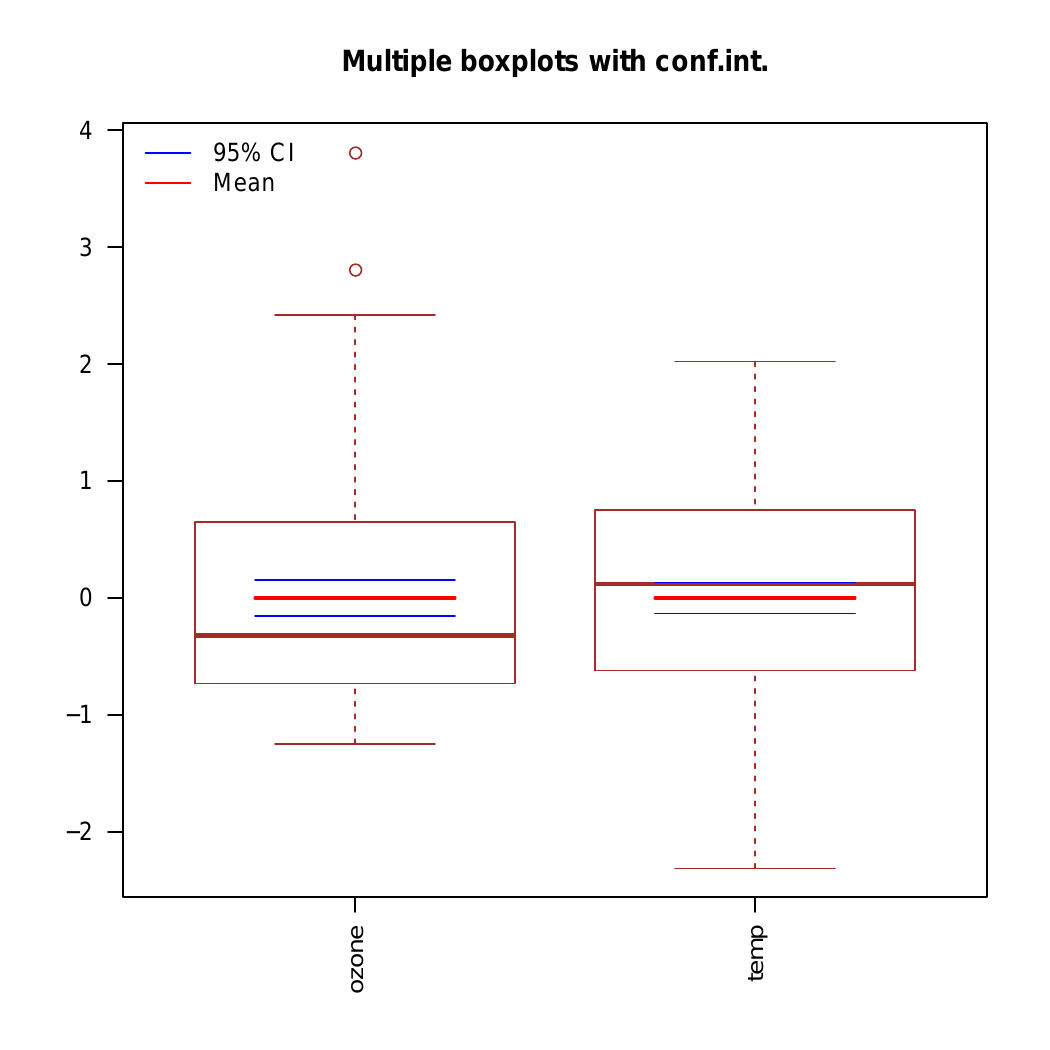
Fig. 38. Example of data representation as box plot with average value and confident interval for normalize data. |
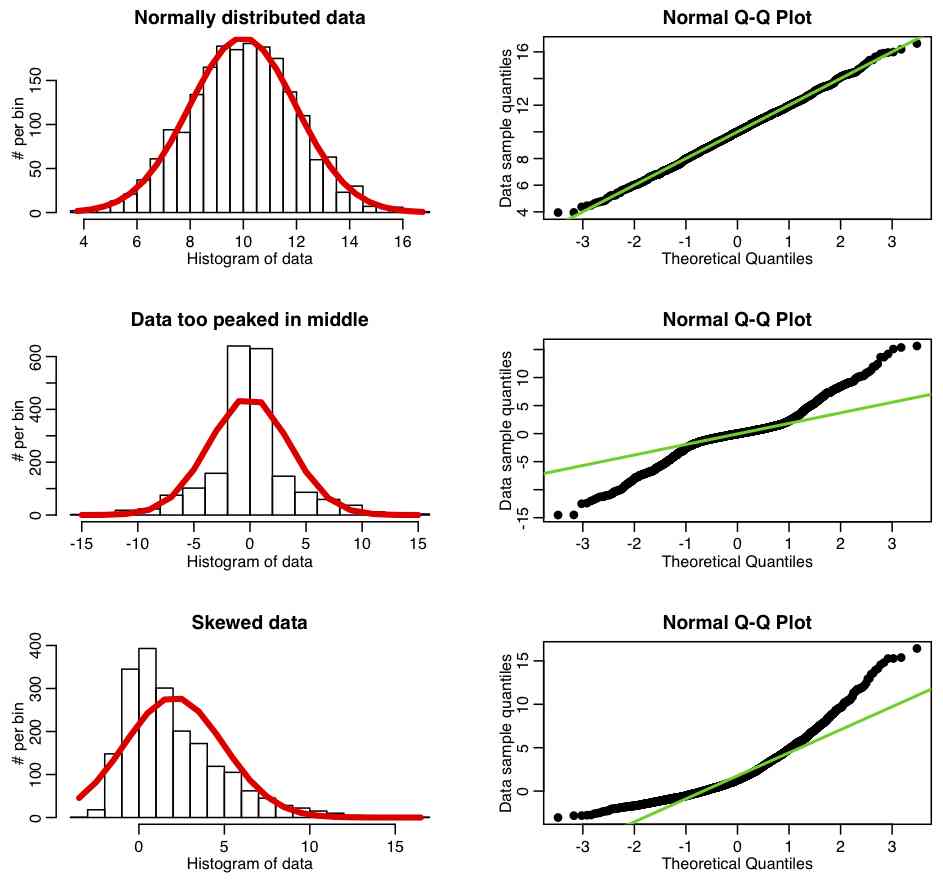
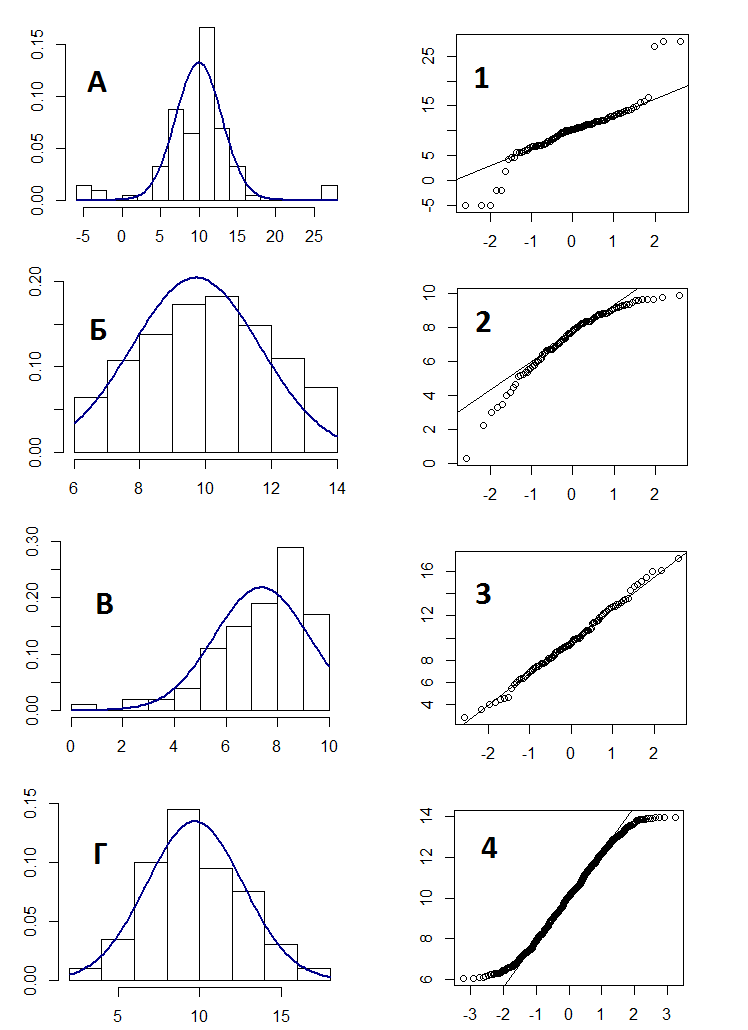
3.3.7 Normality data check
|
Fig. 39. Example of normality check with qq plot (more examples you can find in internet with "qq plot with distribution example" search) |
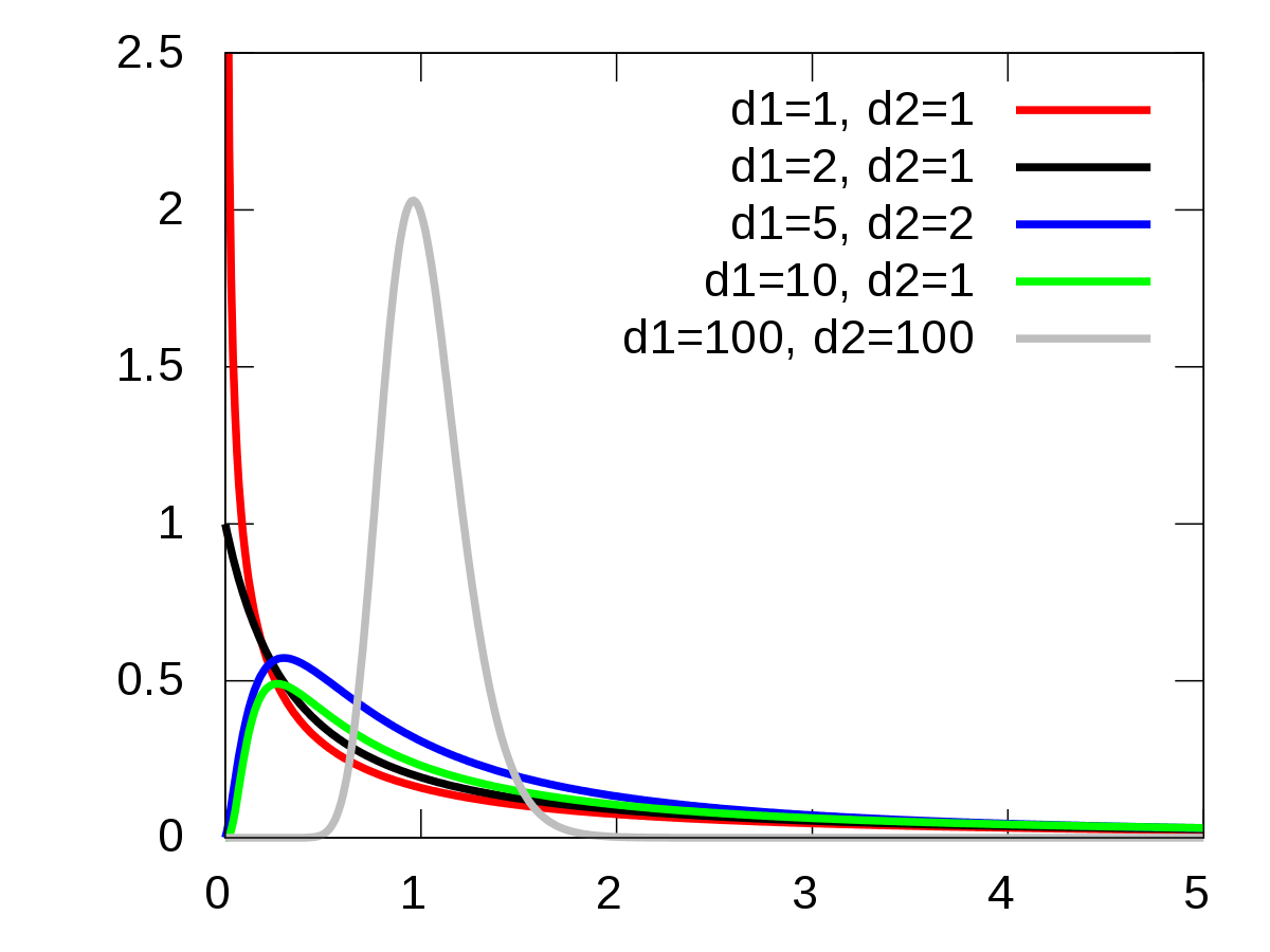
3.3.8 Samples analysis
|
Fig. 40. F-distribution (picture is taken from en.wikipedia.org) |
3.3.9 Multiple comparison

|
Fig. 41. Example of multiple comparison effect from https://xkcd.com. |
3.4 Questions
|
Fig. q-1. |
|
Fig. q-2. |
4. Making accurate models. Analytical practice.
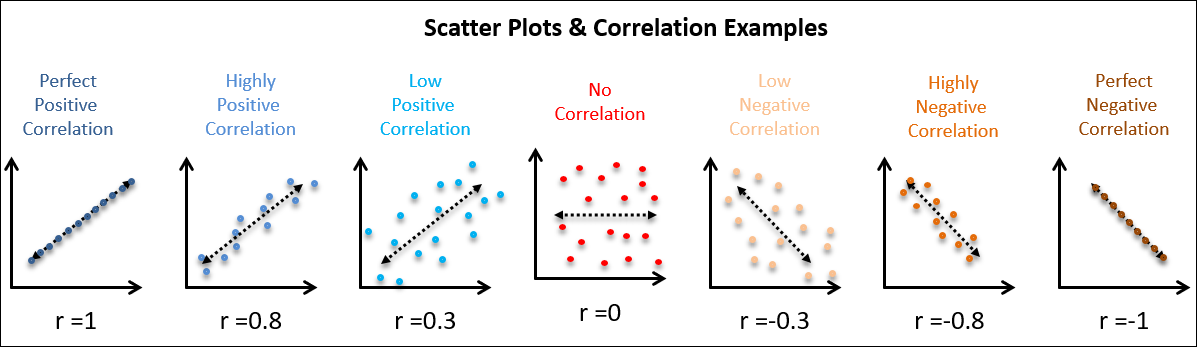
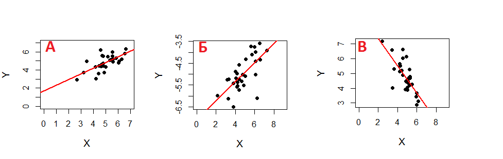
4.1 Correlation
|
Fig. 42. Correlation examples of 2 values from CQE Academy. |
|
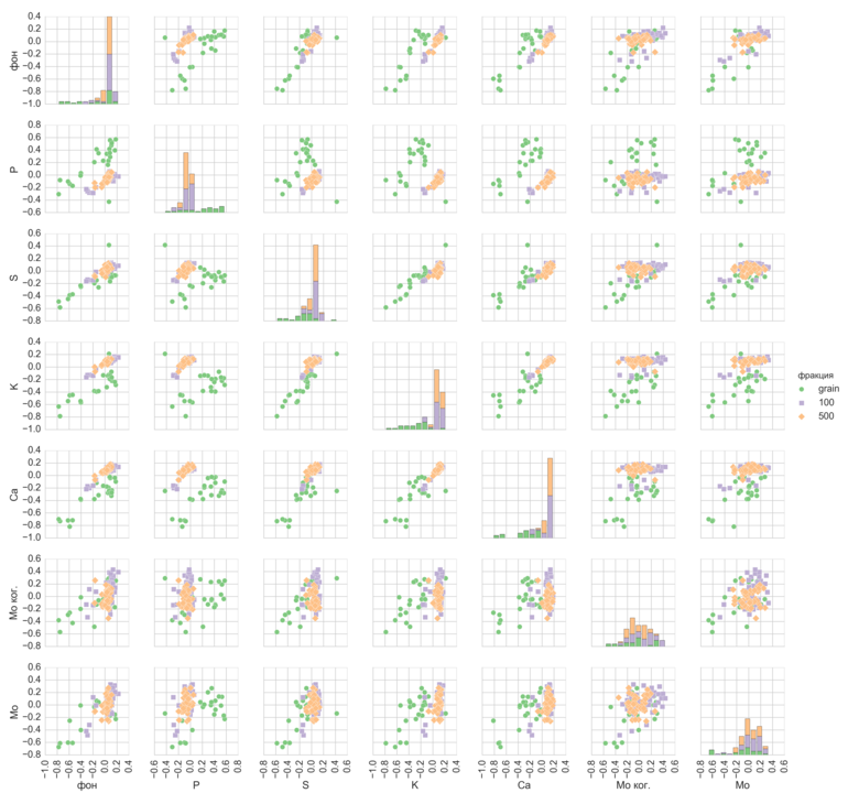
Fig. 43. Example of features binary comparison for 3 type of objects in data science practice. |
|
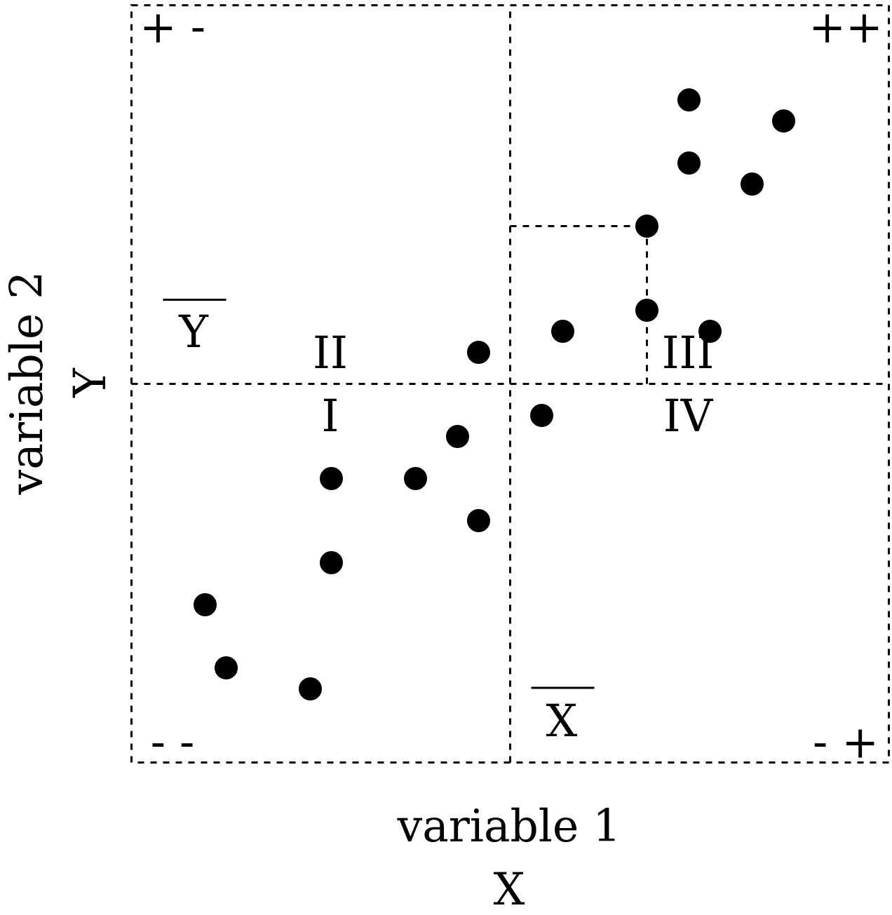
Fig. 44. Correlation coefficient calculation. |
4.2 One variable regression
|
|
Fig. 44. Working principle of Least Square Methods for Linear Regression. |
4.3 Coefficient of determination
4.4 Conclusion
4.5 Questions
|
Fig. q-3. |
|
Fig. q-4. |
References
- Course Experimentation for Improvement from coursera.org.
- Peter Goos, Bradley Jones. Optimal Design of Experiments. A Case Study Approach.
- Book for course Experimentation for Improvement from coursera.org.
- Tutorial for designing experiments using the R package.
- Learning R on simple examples.
- I.A. Rebrova. Experiment planning (in Russ.). 2017. 107 p..
- Course "Basic os Statistic. Part 1" from stepic.org (in Russ.).
- Specialization "Machine Learning and Data Analysis" from coursera.org (in Russ.).
- Course STAT 503 Design of Experiments. Department of Statistics. PennState Eberly College of Science.
- Some information about quantiles and ranks.
- Good linear regression explanation with MS Exel example.
- Confidence interval.
- Christian, Gary D. Analytical chemistry.
- A lot of interesting materials from MSU Chemistry department (in Russ.).
- Models of experiments from 2nd part of this course.